Topology-Aware Uncertainty for Image Segmentation
Notes
- Link to the code here
Highlights
- The authors propose a novel method to estimate uncertainty for curvilinear structures segmentation.
- Unlike other methods the uncertainty map obtained is not pixel-wise but structures-wise.
- The proposed method estimates both inter-structural and intra-structural uncertainty
Introduction
Medical segmentation is by nature ambiguous. Therefore, deep-learning models should capture the uncertainty to give meaningful outputs and help the interpretation of the expert. (see this post). For example, in many vessel segmentation pipelines the segmentation output of an automatic algorithm is proofread by an expert to obtain the final segmentation. In such pipeline the uncertainty map can help the annotator expert to focus on uncertain parts of the segmentation and then facilitate this process.
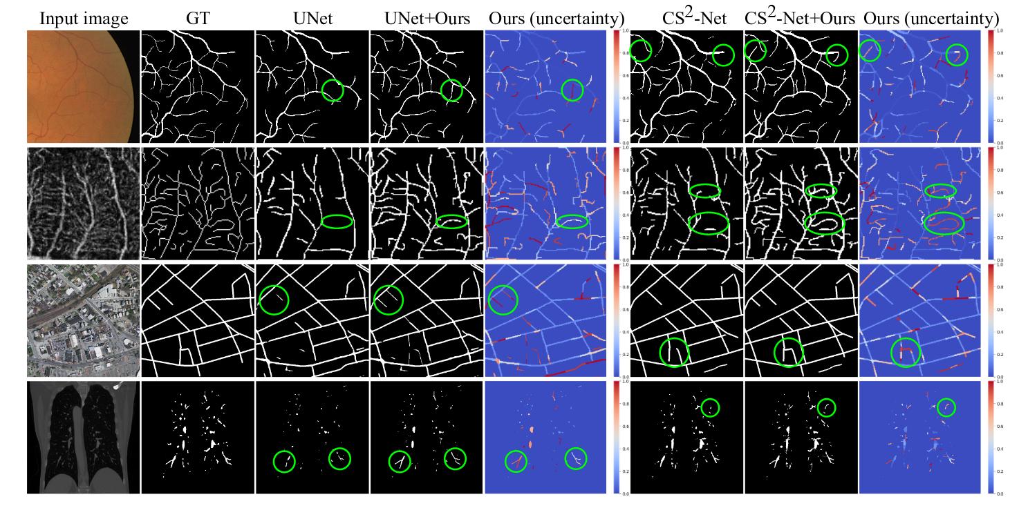
However, existing uncertainty estimation methods do not apply to curvilinear structure segmentation. Indeed, they compute the uncertainty in a pixel-wise manner, generating an uncertainty map highlighting pixels along the boundary of vessels (see Fig.1). Such an uncertainty map is of limited interest for human annotators , this is why the authors proposed a method to compute the uncertainty at a structural level (a structure is a portion of vessel).
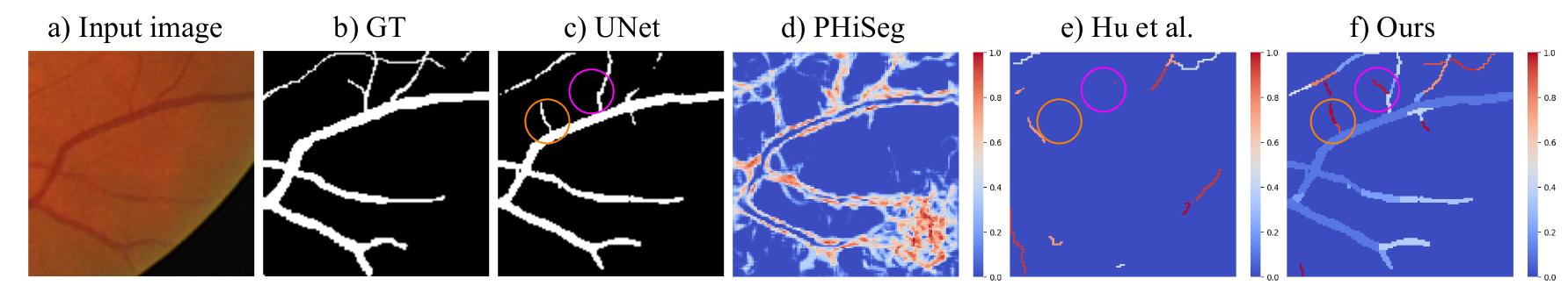
Figure 1: Illustration of the motivation behind the proposed method.
Method
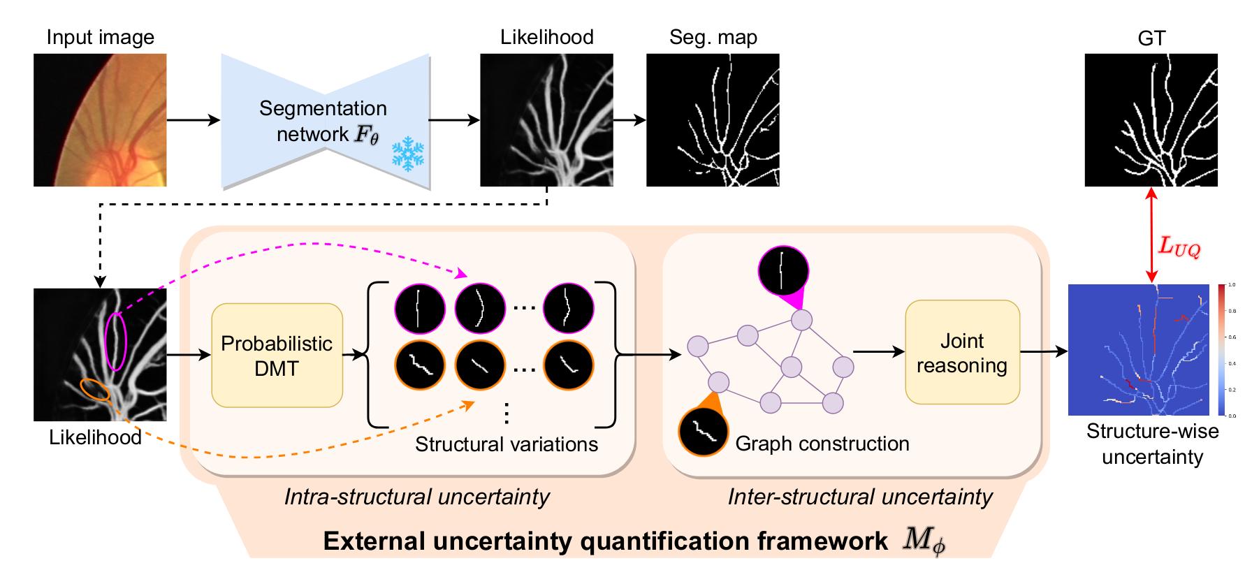
Figure 2: Overview of the method
The proposed framework \(M_{\phi}\) takes in input the original image and the likelihood output of a given segmentation network \(F_{\theta}\). It is composed of a first module, named Probabilistic DMT (Prob. DMT) which goal is to capture the intra-structural uncertainty. The second module is designed to capture the inter-structural uncertainty.
Probabilistic DMT
Prob. DMT is based on the discrete morse theory (DMT) which is explained below.
Discrete Morse theory. DMT treats the likelihood map f as a terrain function, decomposing it into a Morse complex consisting of critical points and paths connecting them. Critical points are locations with gradient equal to zero (minima, maxima and saddle points). V-paths are the routes connecting critical points via the non-critical ones. A V-path connecting a saddle point to a maxima is called a stable manifold. In this paper, the authors only focus on the zero- and one dimensional Morse structures, i.e., the union of all stable manifolds and their associated saddle and maxima. The obtained structure is called the Morse skeleton (see Fig. 3).
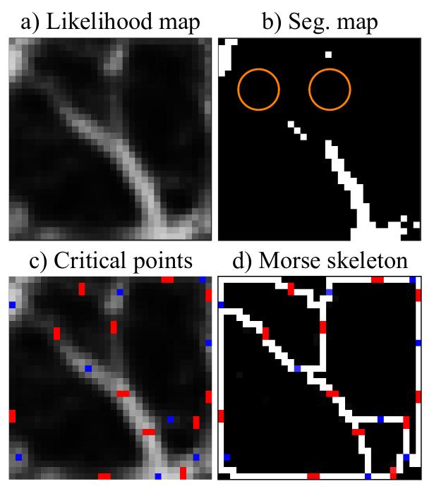
Figure 3: Illustration of the Morse skeleton obtained with the discrete morse theory
This process is entirely deterministic, therefore the authors propose a stochastic version called the Probabilistic DMT.
Probabilistic DMT. To make the generative process stochastic, the authors proposed a perturb and walk algorithm. The likelihood function is perturbed by a random noise and a skeleton is sampled.
Formally, we consider a structure \(e\) obtained following a V-path \((c_s, c_m)\) in the likelihood function \(f\). To generate a variation \(\hat{e}\) of the structure, a likelihood function \(f_n\) is drawn from a distribution centered on \(f\) :
\[f_n \sim f + r\]with \(r\) a random perturbation (Gaussian noise in this work).
With \(f_n\) a new path is generated between \((c_s, c_m)\). The iterative algorithm starts from \(c_s\) and ends at \(c_m\). Two criteria are used to choose the next pixel location: the probability in \(fn\) of the neighborhood pixels and the distance to the destination \(c_m\).
If we consider \(c\) the current pixel location of the walk, the next location \(c''\) is chosen as \(c''=argmax(Q(c'))\), with \(c'\) a neighbor pixel, \(Q(c')=\gamma Q_{d}(c') + (1 - \gamma)f_{n}(c')\), \(Q_{d}(c')=\frac{1}{\vert \vert c_{m} - c' \vert \vert_{2}}\) and \(\gamma\) a hyperparameter.
The \(Q_{d}(c')\) penalty is necessary to avoid the walk to diverge away from \(c_m\).
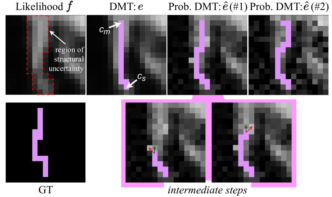
Figure 4: Illustration of the Prob. DMT sampling process.
This process is illustrated in Fig. 4.
By repeating this operation one can sample several instances of a structure capturing the intra-structural uncertainty.
Inter-structural uncertainty
The Prob. DMT module gives a set \(E\) of structures. The second module takes in input each structure \(e \in E\) and outputs the probability of being positive and the uncertainty of \(F_{\theta}\) in the prediction.
The structures are not independent of each other, therefore it is important to consider the spatial context to capture the inter-structural uncertainty.
Here the authors use a Graph Convolution Network (GCN) to model the spatial interactions. Each node represents a structure and edges between nodes exist if the structures are connected.
The input feature for each node is constructed as follows:
Crops centered around the structure are derived from the original input \(x^{c}\), the likelihood feature map \(f^{c}\) and a binary map indicating the presence of the structure \(m\). These crops are then concatenated and passed through convolution blocks and a channel-wise pooling. The persistence value (difference of function values between saddle point and maxima) is also concatenated to the resulting vector. This process is illustrated in Fig. 6.
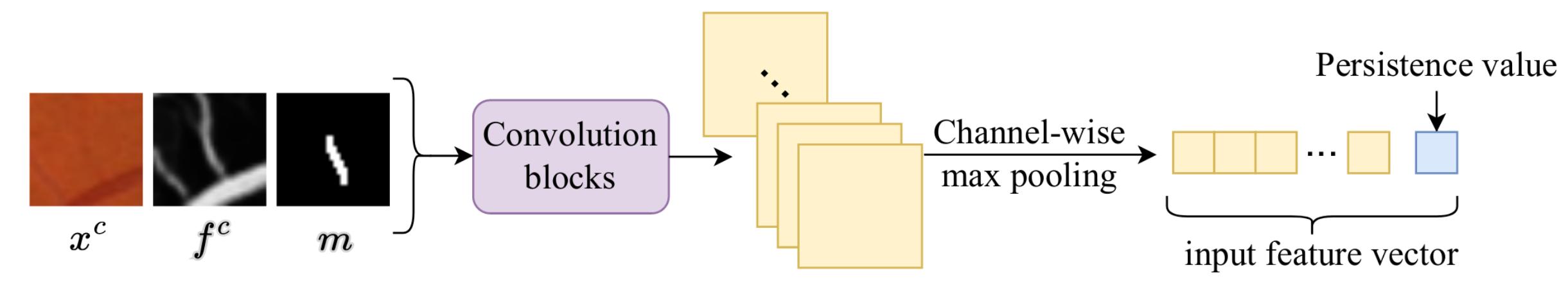
Figure 6: Construction of the input feature vector for each node.
Training the network
The network is trained using the attenuation loss proposed in [¹]. The likelihood output is no longer deterministic but it is modeled as a Gaussian and the variance \(\hat{\delta}^{2}\) of the Gaussian is used as a measure of uncertainty. The network outputs \(\hat{p}(e)\) the probability of being positive and the associated uncertainty \(\hat{\delta}^{2}_{e}\) .
Note : For numerical stability the log variance is predicted \(s_{e}=log \hat{\delta}^{2}_{e}\).
The loss is defined by:
\[L_{UQ}(\phi)=\frac{1}{\vert E \vert}\sum_{e \in E} (\frac{1}{2} \frac{\vert \vert \hat{p}(e) - z_{e} \vert \vert^{2}}{exp(s_{e})} + \frac{1}{2}s_{e})\]with \(z_{e}=(\sum y \odot m) /(\sum m)\), and \(y\) the ground truth.
Proposed module \(M_{\phi}\)
To use the attenuation loss \(M_{\phi}\) must be a probabilistic network. The Prob. DMT is already stochastic and the authors use MC dropout to make the regression network probabilistic.
Inference procedure. \(T\) runs of \(M_{\phi}\) are performed and the uncertainty is performed as \(\bar{\delta}_{e}^{2}=\frac{1}{T}\sum^{T}_{t=1}(\hat{\delta}_{e}^{2})_{t}\).
\(\bar{p}_{e}\) is obtained similarly from \(\hat{p}_{e}\)
Note that these probability and uncertainty are related to one structure
To obtain the full segmentation and uncertainty maps, the probabilities and uncertainties of all structures are combined :
\(\bar{p} = \cup \bar{p}_{e}\) and \(\bar{\delta}^{2} = \cup \bar{\delta}{e}^{2}\).
Then \(\bar{p}\) is binarized and combined with the segmentation map from \(F_{\theta}\).
Then the uncertainty values from \(\bar{\delta}^{2}\) are assigned to the full segmentation map using the shortest distance.
This process is illustrated in Fig. 7.
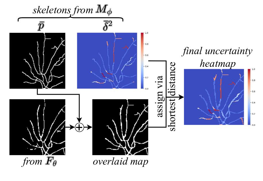
Figure 7: Inference procedure
The method has two outputs :
- the final uncertainty heatmap
- the improved segmentation map
Experiments
- Datasets. 2D retinal vasculature DRIVE, ROSE. 2D aerial images ROADS. 3D CT scans of pulmonary arteries PARSE.
- Baselines. Three types of baselines :
- Vessel Segmentation Method : U-Net, DeepVesselNet, CS2-Net
- Pixel-wise uncertainty estimation methods: Prob-UNet, PHiSeg
- Structure-wise uncertainty estimation method: Hu et al.
- Evaluation metrics.
- Uncertainty quantification: Expected Calibration Error (ECE), Reliability Diagrams (RD)
- Segmentation metrics: DICE, clDice, ARI, VOI, Betti Number error and Betti Matching error
Comparison against uncertainty baselines
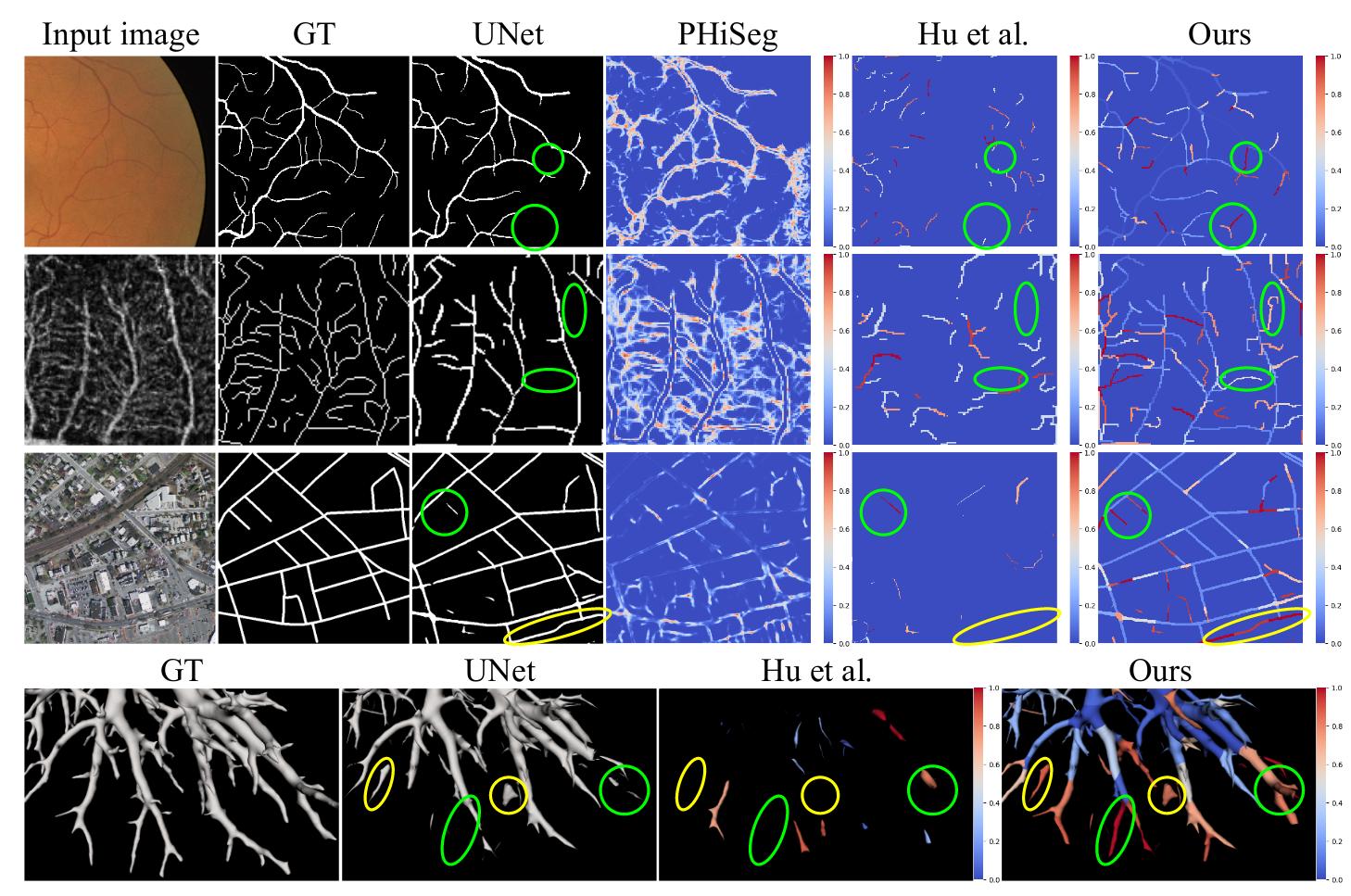
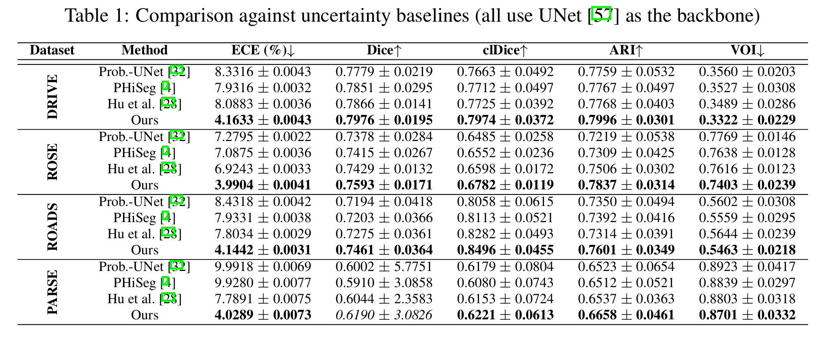
The method is better in terms of calibration (see ECE metrics).
But the most important result is the readability and interpretability of the uncertainty heatmap.
Comparison against segmentation baselines
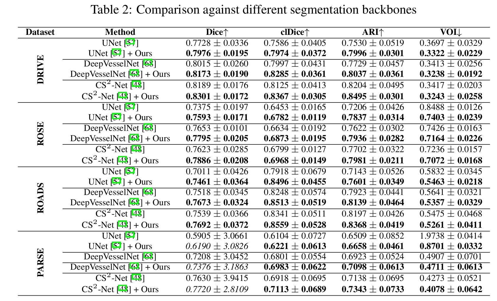
The method improve the segmentation results for all segmentation backbones.
Others results
Performance of proofreading
The authors simulate user interaction. The final segmentation map is given to a user and he inspects structures in decreasing order of uncertainty (till 0.5). He decides to include the structure in the segmentation or not (one ‘click’). The goal is to observe the segmentation improvement with respect to the number of interactions by the users (‘clicks’). The results of this experiment are presented in Fig. 8.
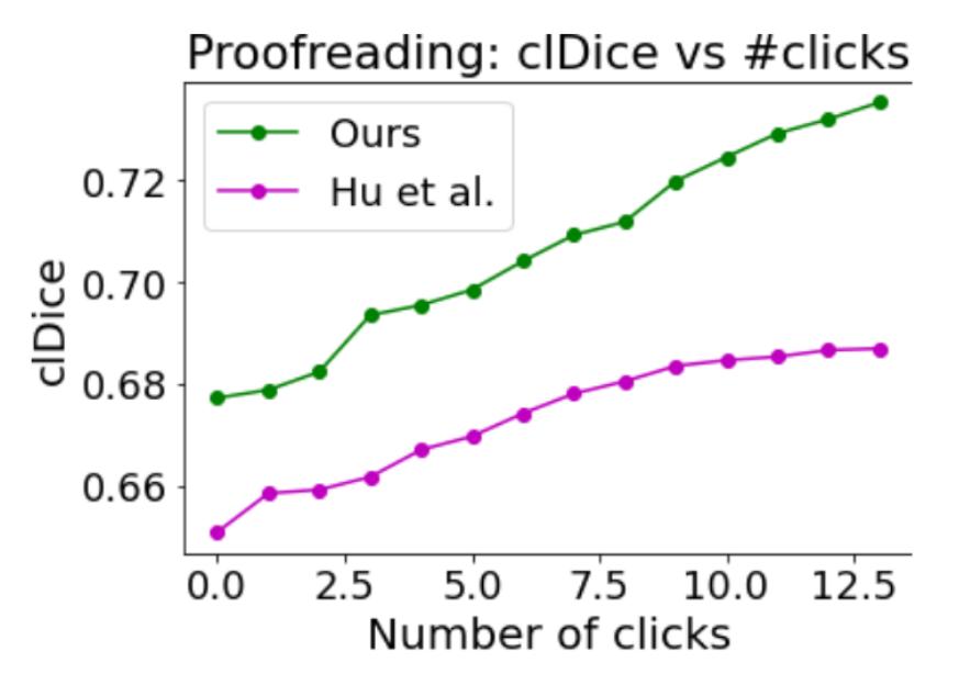
Figure 8: Proofreading experiment
The results show that the method allows the user to fix the segmentation with a small amount of ‘clicks’.
Ablation studies
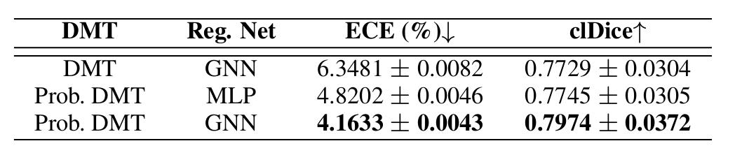
Figure 9: Ablation study
The ablation study shows the importance of the probabilistic framework to capture efficiently the aleatoric uncertainty.
References
[¹] Kendall, A., Gal, Y.: What uncertainties do we need in bayesian deep learning for computer vision? NeurIPS 2017