CoTracker: It is Better to Track Together
Notes
- The official webpage with paper/code/demo
Highlights
- Transformer-based model that tracks dense points in a frame jointly across a video sequence
- Joint tracking results in a significantly higher tracking accuracy and robustness
- Can track arbitrary points, selected at any spatial location and time in the video
- Operates causally on short windows (suitable for online tasks)
-
Trained by unrolling the windows across longer video sequences, which improves long-term tracking
- Introduce the concept of virtual tracks to track more than 70k points jointly and simultaneously
- Introduce the concept of support points to improve performance by jointly tracking additional points to reinforce contextualization
- Introduce the concept of occlusion to track points for a long time even when they are occluded or leave the field of view
Methodology
Context formulation
-
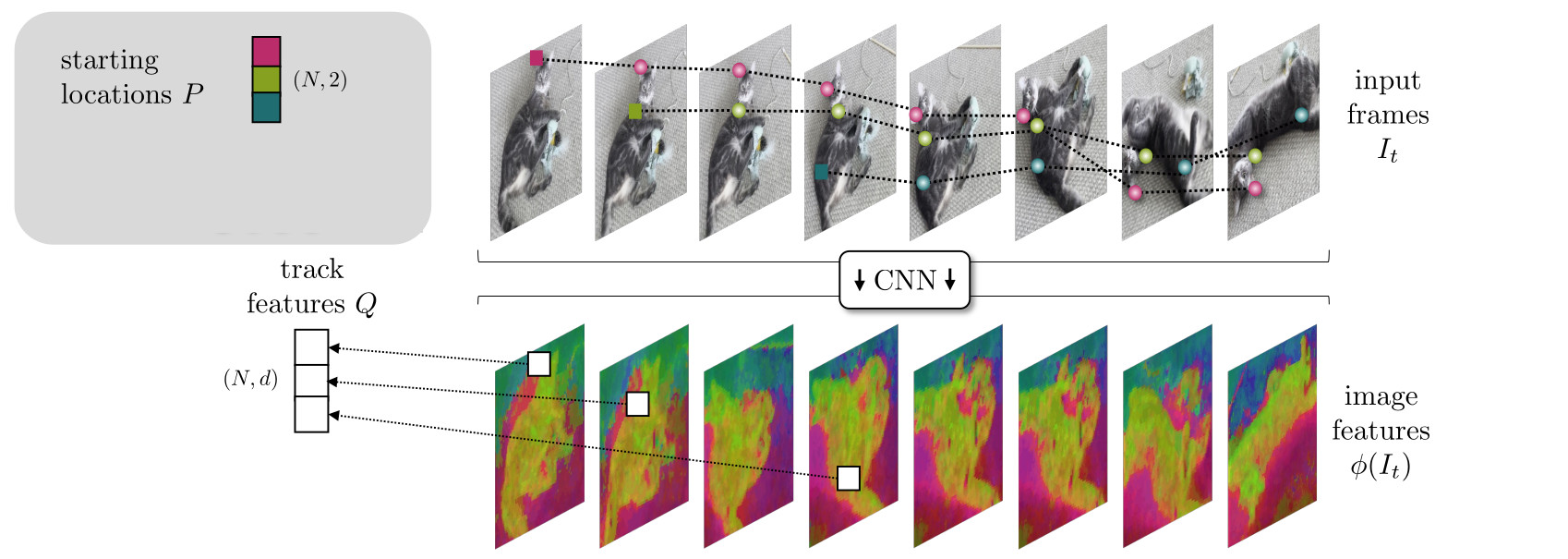
The goal is to track 2D points throughout the duration of a video \(V=\left(I_t\right)_{t=1}^{T}\) composed of a sequence of \(N\) frame \(I_t \in \mathbb{R}^{3 \times W \times H}\)
-
CoTracker predicts \(N\) point tracks \(P_t^i\), with
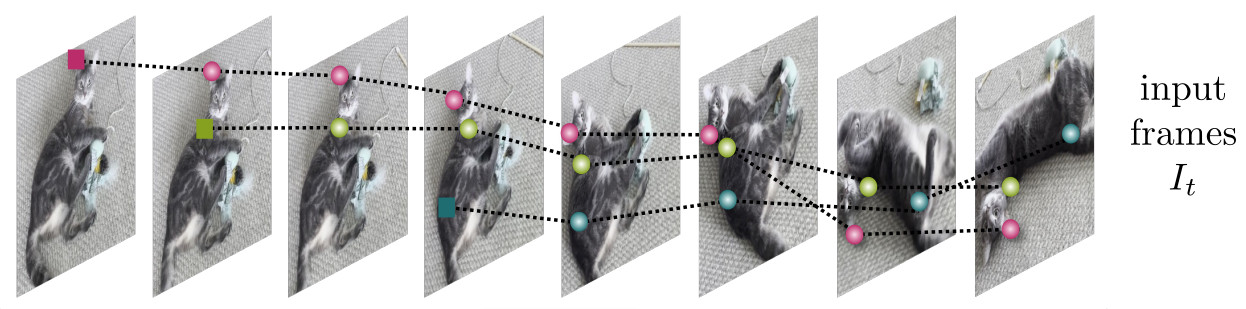
- CoTracker also estimates the visibility flag \(\nu_i \in \{0,1\}\) which tells if a point is visible or occluded in a given frame
Information extaction
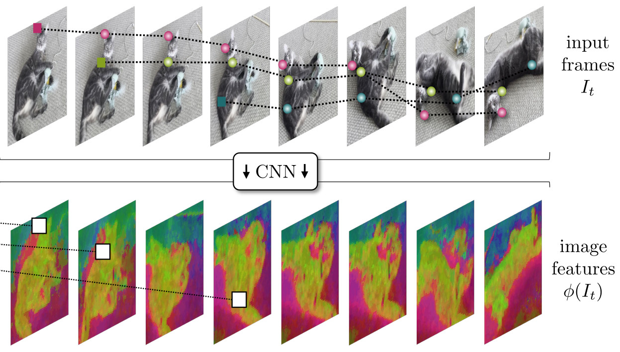
1) Image features
-
\(\phi(I_t) \in \mathbb{R}^{d \times \frac{H}{4} \times \frac{W}{4}}\) are d-dimensional appearance features that are extracted from each video frame using a CNN which is trained end-to-end.
-
The resolution is reduced by a factor of \(4\) for efficiency
-
\(\phi_s(I_t) \in \mathbb{R}^{d \times \frac{H}{4 \cdot 2^{s-1}} \times \frac{W}{4 \cdot 2^{s-1}}}\) are scaled versions of the appearance features used to compute correlation features
-
\(s \in \{ 1, \cdots, S \}\) with \(S=4\) in their implementation
2) Appearance features
-
\(Q_t^i \in \mathbb{R}^d\) are appearance features of the tracks
-
They are time dependent to accommodate changes in the track appearance
-
They are initialized by sampling image features \(\phi(I_t)\) at the starting locations
-
They are updated by the transformer
3) Correlation features
-
\(C_t^i\) are correlation features which are computed to facilitate the matching of the point tracks
-
Each \(C_t^i\) is obtained by comparing the track features \(Q_t^i\) to the image features \(\phi_s\left(I_t\right)\) around the current estimate \(\hat{P}_t^i\) of the track’s location
-
The vector \(C_t^i\) is obtained by stacking the inner products \(\left<Q_t^i,\phi_s\left(I_t\right)\left[ \hat{P}_t^i /(4 \cdot s) + \delta \right] \right>\)
-
\(s \in \{1,\cdots,S\}\) are the feature scales
-
\(d \in \mathbb{Z}^2\), \(\|\delta\|_{\infty} \leq \Delta\) are offsets
-
The image features \(\phi_s\left(I_t\right)\) are sampled at non-integer locations by using bilinear interpolation and border padding
-
The dimension of \(C_t^i\) is \((2\Delta+1)^2S = 196\) with \(S=4\) and \(\Delta=3\)
Transformer formulation
General framework
-
CoTracker is a transformer \(\Psi : G \rightarrow O\) whose goal is to improve an initial estimate of tracks
-
The input \(G\) corresponds to a grid of input tokens \(G_t^i\), one for each point track \(i \in \{1, \cdots N \}\) and time \(t \in \{1,\cdots,T \}\)
-
The output \(O\) is a grid of output tokens \(O_t^i\) which are used to update the point tracks during iterations
Input tokens
- The input tokens \(G(\hat{P},\hat{\nu},\hat{Q})\) code for position, visibility, appearance, and correlation of the point tracks and is given as:
-
\(\eta(\cdot)\) is a positional encoding of the track location with respect to the initial location at time \(t=1\)
-
\(\eta'(\cdot)\) is a positional encoding of the start position \(\hat{P}_1^i\) and for time \(t\), with appropriate dimensions
-
The estimates \(\hat{P}\), \(\hat{\nu}\) and \(Q\) are initialized by broadcasting the initial values \(P_{t_i}^{i}\) (the location of query point), \(1\) (meaning visible) and \(\phi\left(I_t\right)[P_{t_i}^{i}/4]\) (the appearance of the query point) to all time \(t \in \{1,\cdots,T\}\)
![]()
Output tokens
- The output tokens \(O\left( \Delta \hat{P}, \Delta Q \right)\) contains updates for location and appareance, i.e. \(O_t^i = \left( \Delta \hat{P}_t^i, \Delta Q_t^i \right)\)
Iterated transformer applications
-
The track estimates are progressively refined using an iterative process \(m \in \{0,\cdots,M\}\)
-
\(m=0\) denotes initialization
-
Each update computes
-
The visibility mask \(\hat{\nu}\) is not updated by the transformer but once after the last \(M\) applications of the transformer using the appearance features as \(\hat{\nu}^{(M)} = \sigma\left(W Q^{(M)}\right)\)
-
The transformer \(\Psi\) interleaves attention operators that operate across the time and point track dimensions, so to reduce the complexity from \(O( N^2 T^2)\) to \(O( N^2 + T^2 )\)
-
Virtual tracks concept is introduced to even reduce the complexity when \(N\) is large
-
Virtual tracks tokens are simply added as additional tokens to the input grid with a fixed, learnable initialization and removed at the output
-
\(K\) virtual tracks tokens reduce the complexity to \(O( NK + K^2 + T^2 )\)
![]()
Training process
-
Use of sliding window concept to handle long videos of length \(T'>T\), where \(T\) is the maximum window length supported by the architecture
-
The videos are split in \(J = [2T'/T-1]\) windows of length \(T\), with an overlap of \(T/2\) frames
-
A first loss is used for track regression
-
where \(\gamma=0.8\) discounts for early transformer updates and \(P^{(j)}\) corresponds to the ground-truth trajectories restricted to window \(j\)
-
A second loss is the cross entropy of the visibility flags
-
where \(\nu^j\) are the reference visibility flags
-
Use of a simple token masking strategy to deal with points that have not been tracked since the first frame (i.e points with \(t_i > 1\))
Support points
-
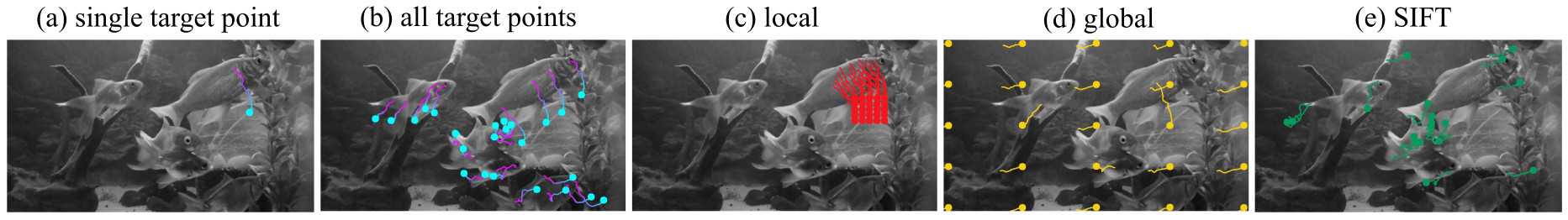
The author found it beneficial to tack additional support points which are not explicitly requested by the user
-
The key idea is to reinforce contextual aspects through the joint tracking formulation
-
Different configuration are tested, with global strategy (support points form a regular grid across the whole image), with local strategy (the grid of points is centered around the point we wish to track, allowing the model to focus on a neighbourhood of it), or with SIFT strategy (SIFT is used to detect support points)
Experiments
Datasets
-
TAP-Vid-Kubrik: synthetic dataset used for training. It consists of sequences of 24 frames showing 3D rigid objects falling to the ground truth under gravity and bouncing
-
TAP-Vid-DAVIS: real dataset used for evaluation. It contains 30 real sequences of about 100 frames. Points are queried non random objects at random times and evaluation assesses both predictions of positions and visibility flags
-
PointOdyssey: Synthetic dataset used for training and evaluation of long-term tracking. It contains 100 sequences of several thousand frames with objects and characters moving around the scene
-
Dynamic Replica: Synthetic dataset for 3D reconstruction used for training and evaluation of long-term tracking. It consists of 500 sequences of 300 frames of articulated models of people and animals used for training and evaluation of long-term tracking.
Metrics
-
OA (\(\uparrow\)) - Occlusion accuracy - accuracy of occlusion prediction treated as binary classification
-
\(\delta_{avg}^{vis} (\uparrow)\) - fraction of visible points tracked within 1, 2, 4, 8 and 16 pixels, averaged over threshold
-
AJ (\(\uparrow\)) - Average Jaccard - measuring jointly geometric and occlusion prediction accuracy
-
Survival rate (\(\uparrow\)) - average fraction of video frames until the tracker fails (detected when tracking error exceeds 50 pixels)
Implementaton details
-
11,000 TAP-Vid-Kubric sequences of \(T'=24\) frames were used for training using sliding window size \(T=8\)
-
50,000 iterations during training using 32 A100 80 GB GPUs !

-
Batch size of 32
-
Learning rate of \(5e^{-4}\) and a linear 1-cycle learning rate schedule, using the AdamW optimizer
-
Training tracks are sampled preferentially on objects
-
During training, construction of batches of 768 tracks out of 2048 among those that are visible either in the first or middle frames of the sequence to train
-
Train the model with \(M=4\) iterative updates and evaluate it with \(M=6\)
Results
Is joint tacking beneficial ?
- TAP-Vid-DAVIS dataset used for tracking using either a single target point at a time or all target point simultaneously
- Different configuration of support points are tested
Table 1 - Importance of joint tracking. Comparison using time and cross-track attention, tracking single or multiple target points, and using additional support points.
How does CoTracker compare to prior work ?
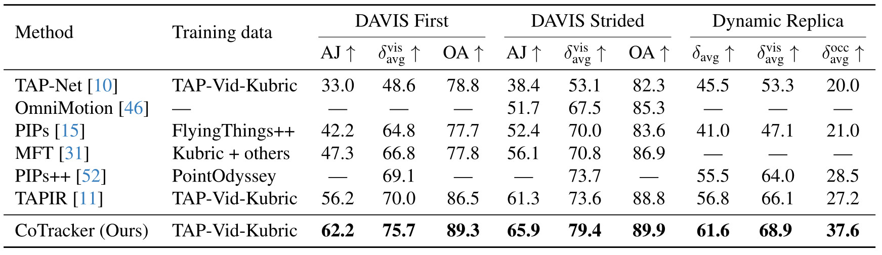
Table 2 - State of the art comparison. CoTracker was compared to the best trackers available on TAP-Vid-DAVIS as well as on Dynamic Replica.
Figure 1 - State of the art comparison. First column: PIPs, second column: RAFT, third column: TAPIR, last column: CoTracker.
Is unrolled training important ?
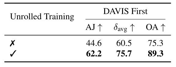
Table 3. Unrolled training. CoTracker is built for sliding window predictions. Using them during training is important.
Do virtual tracks help CoTracker to scale ?
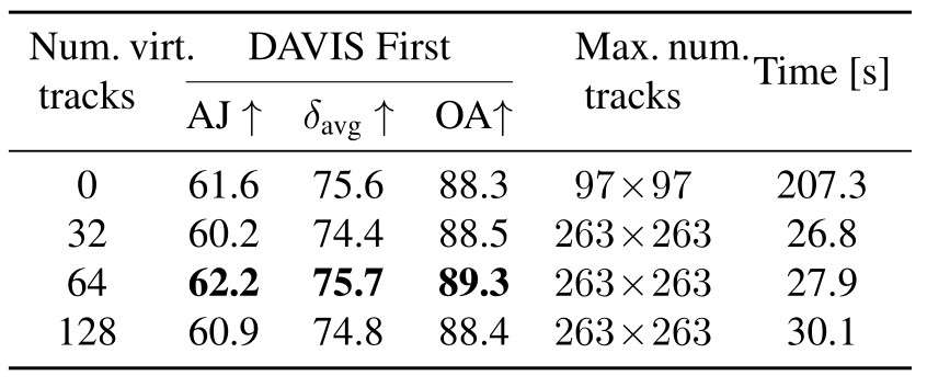
Table 4. The virtual tracks allow CoTracker to scale. We report the maximum number of tracks that can fit on a 80 GB GPU.
Conclusions
- Joint tracking of points improves results
- CoTracker is among the current best performing method for point tracking
- Introduce several interesting concepts, such as occlusion flags and support points