VT-ADL: A Vision Transformer Network for Image Anomaly Detection and Localization
Context
- Anomaly detection, also called outlier detection or one-class classification, is the process of detecting events/items that deviate significantly from the normality. A distribution of the normal class is estimated and the event/item is said to be anomalous if it does not belong to this distribution.
- Here we tackle the problem of anomaly detection in images in the context of machine learning, meaning we will train a network (or another kind of algorithm) on normal images only, and then, at inference, we will try to classify images as normal VS anomalous.
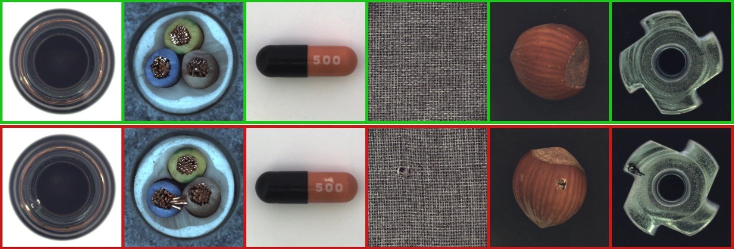
Example of normal (green) VS anomalous (red) image on the MVTecAD dataset - The objective of this paper is to propose an anomaly detection method which make use of a transformer, a decoder and a Gaussian Mixture Model (GMM) estimation network.
- The authors also introduce a database similar to MVTecAD, containing 3 objects named BTAD.
Highlights
- Combination of transformer, decoder and GMM for anomaly detection.
- Introduction of a new “MVTec like” dataset named BTAD.
Methods
The model is divided in 3 blocks :
1) Transformer-encoder
1.a) Transformer
The transformer architecture is the same as in the original ViT paper. The image is decomposed in patches, embedded through a linear layer, summed with a position embedding and then passed through multiple encoding layers.
\[\mathbb{R}^{H \times W \times C} \xrightarrow[\text{division}]{\text{patch}} \mathbb{R}^{N \times P \times P \times C} \xrightarrow[\text{layer}]{\text{linear}} \mathbb{R}^{N \times D} \xrightarrow[\text{}]{\text{transformer}} \mathbb{R}^{N \times D}\]With \(H \times W\) the size of the base image, \(C\) the channel size, \(P \times P\) the patch size and \(N\) the number of patch.
The reduction operation here is done in the linear projection layer (because \(D > P \times P \times C\), this is not always the case).
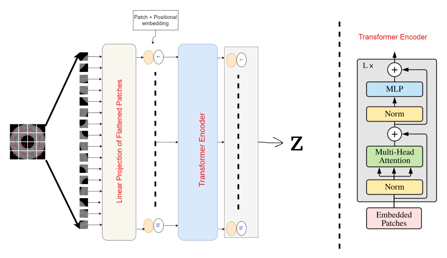
Note : In the paper the authors mention a dimension \((N+1)\) as if there is a class token, but I saw no use of a class token, nor do they speak about it, so I think the dimension is \(N\) and not \((N+1)\).
1.b) Encoder
After the transformer, the output sequence is reduced in dimension again before being fed to the decoder. The authors used a linear projection step. They also mention a sum of the sequence, so both might be feasible and operate the same dimension reduction.
\[\mathbb{R}^{N \times D} \xrightarrow[\text{projection}]{\text{linear}} \mathbb{R}^{D}\]2) Decoder
The decoder is a classical CNN decoder, consisting of 5 transposed convolutional layers, with batch-normalization and ReLu activation, except for the last layer which uses tanh activation. The 1D vector is first reshaped as a 2D matrix.
\[\mathbb{R}^{D} \xrightarrow[\text{ }]{\text{decoder}} \mathbb{R}^{N \times P \times P \times C}\]3) GMM estimation
The GMM estimation network, uses as input the output of the transformer (1.a), i.e. the sequence output by the transformer.
The goal is to estimate the mixture weights, means and variance of the GMM, which will be output by the network.
Then given the data samples and the estimated distribution, one can compute the negative log likelihood (NLL) of each sample.
Note : this process is different than the “usual” process consisting for a network to output the membership of each sample, and then analytically determining the mixture weights, means and variances.
Also note that here \(K = 150\)
Global view :
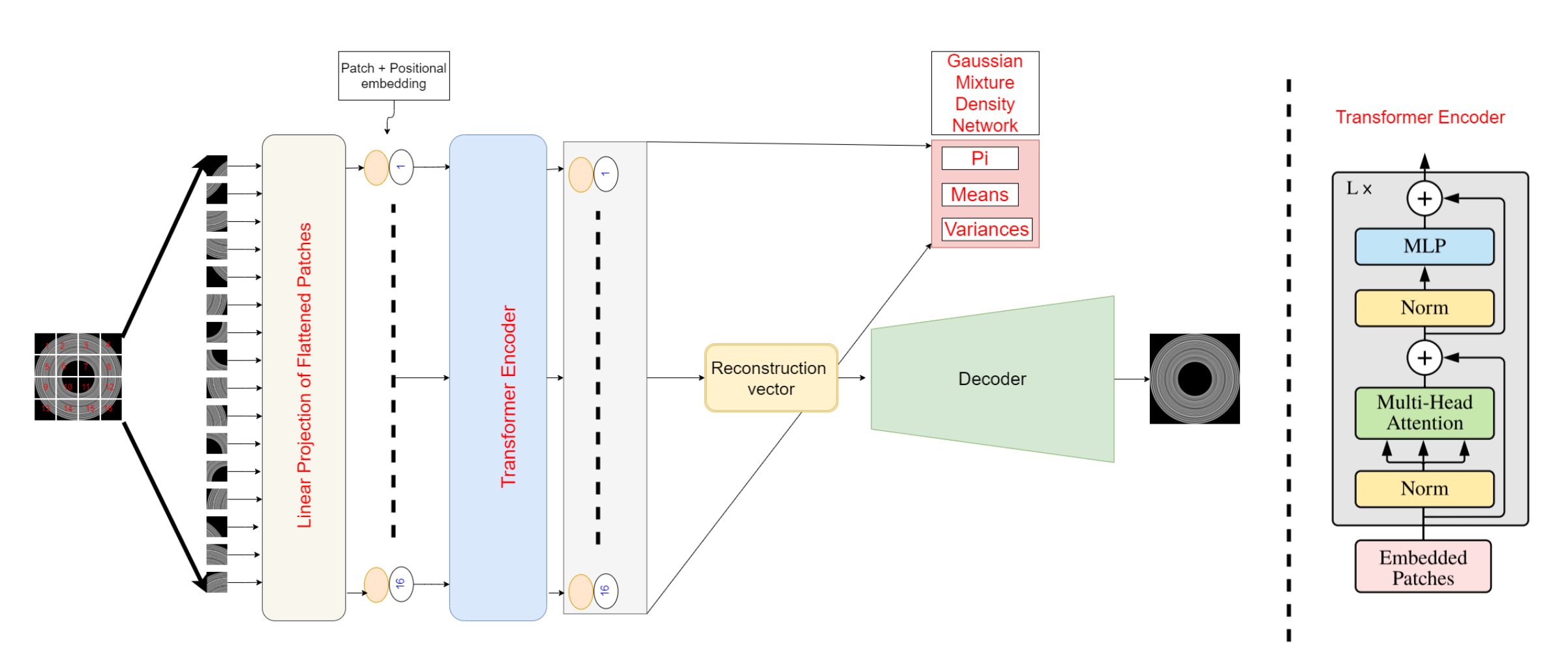 After inspection of the code on github we found : \(H = W = 512\), \(P = 32\), \(N = \frac{HW}{P^2} = 256\), \(D = 512\) (which is a coincidence that it is equal to \(H\) and \(W\)).
Loss (training/testing) :
The loss function consists of three terms to balance, two to measure the quality of the reconstruction error (the \(l_2\) norm and the structural similarity) that affects the transformer, encoder and decoder, and a third term (NLL) that affects the transformer and the GMM estimation network.
\[L(x) = NLL(GMM(\text{transformer}(x))) + \lambda_1 ||x - \hat{x}||_2^2 + \lambda_2 SSIM(x, \hat{x})\]With \(\hat{x} = \text{decoder(encoder(transformer(}x\text{)))}\).
At inference stage, to perform anomaly detection (is there an anomaly in the image ?) the authors used the same loss as in the training.
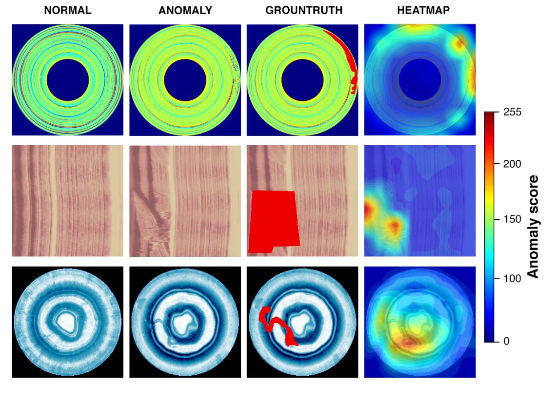
To perform anomaly localization (where is the anomaly in the image ?) the authors used only the NLL obtained for each patch, that was then upsampled using bilinear interpolation.
Results
Anomaly detection (is there an anomaly in the image ?)
The authors report SOTA results on MNIST (one digit considered normal VS the 9 others)

Anomaly localization (where is the anomaly in the image ?)
The authors report SOTA results on MVTec.


The authors also introduce their model performance on the BTAD database that they introduced.
Conclusions
The authors introduced a database that shares many similarities with MVTecAD, thus being smaller.
They also introduce an anomaly detection model consisting of a transformer, a decoder and a gaussian mixture model estimator. It cleverly combines these 3 blocks to achieve SOTA performance on anomaly detection tasks (MNIST, MVTec) and anomaly localization tasks (MVTec).
BTAD dataset.