Momentum Residual Neural Networks
Reminder on Residual Neural Networks
Seminal work on Residual Neural Network : “Deep Residual Learning for Image Recognition”, K. He, X. Zhang, R. Zen and J. Sun, CVPR 2016
Main points:
- Deeper neural networks are more difficult to train.
- Residual learning framework has been introduced to ease the training of deeper networks.
- Layers are reformulated as learning residual functions with reference to the previous layer inputs, instead of learning unreferenced functions.
- These residual networks are easier to optimize, and can gain accuracy from considerably increased depth.
Highlights of the paper
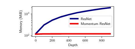
- Exploration of memory costs issues in residual neural network due to backpropagation schemes.
- Proposition of a new model, Momentum ResNets, which circumvents these memory issues by being invertible.
- Compared to other invertible models, this model is simple to integrate into the usual ResNets architectures and provides a rigorous mathematical setting.
- Momentum ResNets can be interpreted as second order ordinary differential equations (ODEs).
- Momentum ResNets separate point clouds that ResNets fail to separate.
Introduction
The main goal of this paper is to explore the properties of a new model, Momentum ResNets, that circumvents the memory issues of ResNets by being invertible. It relies on the modification of the ResNet’s forward rule.
Momentum Residual Neural Networks
Backpropagation, used to optimize deep architectures, requires to store values at each layer during the network training. In classical ResNets, we have the feedforward relation:
\[x_{n+1}=x_n+ f(x_n,\theta_n)\]where \(\theta_n\) is the set of parameters, and \(x_n\) the activations at layer \(n\).
Memory issues occur when increasing the number of layers.
The authors propose to use momentum equations that replace the classical relation above:
\[v_{n+1}=\gamma v_n+(1-\gamma)f(x_n,\theta_n)\] \[x_{n+1}=x_n+v_{n+1}\]where \(v\) is a velocity term and \(\gamma\) a momentum term.
The method consists in modifying the forward equations using the same parameters as inputs. This is invertible since we can recover the values of \(x_{n}\) and \(v_{n}\) using \(x_{n+1}\) and \(v_{n+1}\). If we invert these equations, we get :
\[x_n=x_{n+1}-v_{n+1}\] \[v_n=\frac{1}{\gamma} (v_{n+1}-(1-\gamma)f(x_n,\theta_n))\]This avoids the memory issues occurring due to the backpropagation step.
Note: Momentum gradient descent is an alternative to classical gradient descent algorithms using second order partial derivatives. An overview of gradient descent optimization algorithms is given in a review by S. Ruder, referenced in the paper.
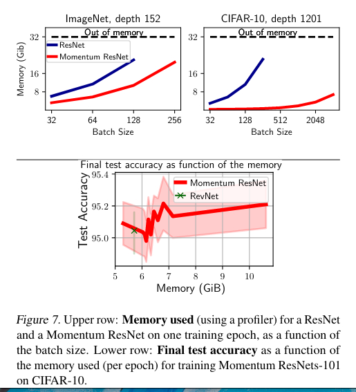
Memory cost
For usual ResNets, one needs to store the weights of the network and the values of all activations for the training set at each layer. The memory needed is \(O(k*d*n_{batch})\) while for the Momentum ResNets the memory need is \(O((1-\gamma)*k*d*n_{batch})\) where \(k\) is the depth of the network, \(d\) the size of the vector \(x\), and \(n_{batch}\) the size of the training set.
The role of momentum
When \(\gamma=0\), they get a Classical ResNet. When \(\gamma \rightarrow 1\), they get a special case of the invertible RevNet (Gomez et al, 2017).
The advantage of the Momentum ResNet compared to RevNet, where two learnable functions are used, is its stability for convergence (proofs given in the paper).
Link with ODE (Ordinary Differential Equations)
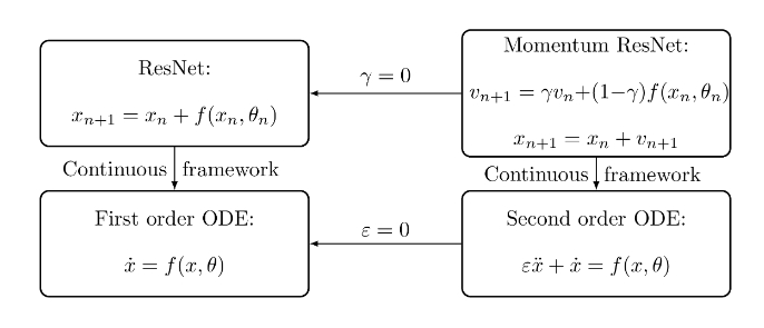
ResNets can be interpreted as a first order ODE. Indeed, the term \(x_{n+1} - x_n\) can be seen as the discretized partial derivative \(\dot{x}\).
\[\dot{x} \quad \rightarrow \quad x_{n+1}-x_{n}\]Momentum ResNets can be interpreted as second-order ODEs by taking \(\epsilon=\frac{1}{1-\gamma}\), they get:
\[v_{n+1}=v_{n} + \frac{f(x_n,\theta_n) - v_n}{\epsilon}\] \[x_{n+1}=x_n+v_{n+1}\]by replacing the term \(v_n\), they find:
\[x_{n+1}-x_{n}=x_n-x_{n-1} + \frac{f(x_n,\theta_n)-v_n}{\epsilon}\]The second order derivative \(\ddot{x}\) can be discretized using \(x_{n+1}-2x_n+x_{n-1}\) and then we can interpret the Momentum ResNets as a second order ODE of the form:
\[\epsilon \ddot{x}+\dot{x}=f(x,\theta)\]“In the same way that ResNets can be seen as discretization of first order ODEs, Momentum ResNets can be seen as discretization of second-order ones.”
When \(\epsilon \rightarrow 0\), they get the first order model.
Representation capabilities
These analogies between ODEs lead to some interesting mathematical properties. The first order model can represent homeomorphism mappings (continuous, bijective with continuous inverse). However, first order ODEs are not universal approximators and some mappings are not possible (see the example on point clouds separation). Momentum ResNets can capture non-homeomorphic dynamics. The authors present some proofs on this aspect called “representation capabilities” of models.
Experiments
Point clouds separation
- Experiments on 4 rings (2 classes) of point clouds
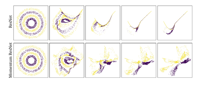
Momentum ResNets are able to separate these classes, whereas classical ResNets fail.
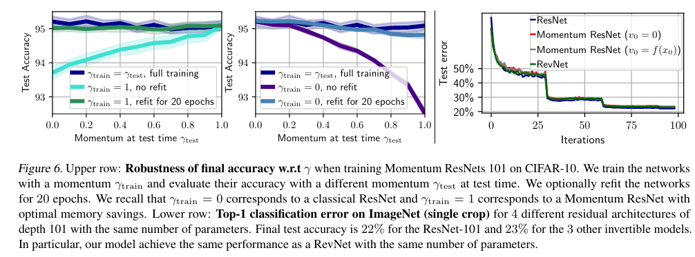
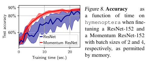
Real data sets
- Database: ImageNet and CIFAR10/100
- Momentum ResNets were used with two different initializations: one with an initial speed \(v_0 = 0\) and the other one where the initial speed \(v_0\) was learned: \(v_0 = f (x_0)\)
- For comparison, the authors use both ResNet-101 (non invertible) and RevNet-101 (invertible model)
They study the accuracy, the effect of the momentum term \(\gamma\), and the memory costs.
Conclusions
- This paper introduces Momentum ResNets, new invertible residual neural networks operating with a significantly reduced memory footprint compared to ResNets.
- In contrast with existing invertible architectures, they propose a simple modification of the ResNet forward rule.
- Momentum ResNets interpolate between ResNets (γ = 0) and RevNets (γ = 1), and are a natural second-order extension of neural ODEs with nice mathematical properties and more generic representation capabilities.
Remarks
- A python package is available here: Momentum GitHub.
- This video is a good presentation of the paper.