Deep Unsupervised Learning using Nonequilibrium Thermodynamics
Notes
- Code is available on GitHub: https://github.com/Sohl-Dickstein/Diffusion-Probabilistic-Models
Introduction
The authors propose a new probalistic model that aims to link a known distribution \(\pi(.)\) to another one \(q(.)\) based on diffusion. To achieve it, they iteratively added small amount of noise on the target distribution until it is converted into the known distribution. This process can be seen has a Markov chain that can be learned reversly.
Highlights
They proposed a new iterative framework that allows:
- To generate data from a known distribution by defining thousands of steps that have a simple functional form.
- To tract changes through data generation using these simple, incremental steps.
- To combine different distributions (e.g. with a conditional distribution, you can do inpainting)
Diffusion probalistic model
“A Markov chain or Markov process is a stochastic model describing a sequence of possible events in which the probability of each event depends only on the state attained in the previous event.” 1
A diffusion probalistic model consists in building a markov chain which allows to switch from a simple known distribution \(\pi(.)\) ( ex : a gaussian distribution ) to a target distribution \(q(.)\) (ex : a kind of image distribution). To obtain that chain they start from the target distribution and add small perturbations thousands of times (eq. time steps) until they obtain the known distribution. This is the forward trajectory.
Forward trajectory
Let
- \(q(\mathbf{x}^{(0)})\) be the data distribution
- \(T_{\pi}(\mathbf{y}\mid\mathbf{y}';\beta)\) be a Markov diffusion kernel
- \(\beta_t\) be a diffusion rate
We can define \(q\left(\mathbf{x}^{(t)} \mid \mathbf{x}^{(t-1)}\right)\) with \(t\) a time step in the Markov chain such as :
\[q\left(\mathbf{x}^{(t)} \mid \mathbf{x}^{(t-1)}\right)=T_\pi\left(\mathbf{x}^{(t)} \mid \mathbf{x}^{(t-1)} ; \beta_t\right)\]Let’s assume that at \(T\) steps, \(q(\mathbf{x}^{(0...T)})\) is converted into the simple distribution \(\pi(.)\). We can define analytically \(q(\mathbf{x}^{(0...T)})\) such as:
\[q\left(\mathbf{x}^{(0 \cdots T)}\right)=q\left(\mathbf{x}^{(0)}\right) \prod_{t=1}^T q\left(\mathbf{x}^{(t)} \mid \mathbf{x}^{(t-1)}\right) = \pi (\mathbf{x}^T)\]However, what is interesting about the method is to be able to convert a simple distribution \(\pi(.)\) into an element included in the unknown \(q(.)\). That is the reverse trajectory.
Reverse trajectory
The Markov chain has been analytically created, therefore the forward trajectory form is known. As changes applied from a time step to another are small, diffusion kernels have the same functional form in both trajectories. Thus we can define :
\[p\left(\mathbf{x}^{(T)}\right)=\pi\left(\mathbf{x}^{(T)}\right)\] \[p\left(\mathbf{x}^{(0 \cdots T)}\right)=p\left(\mathbf{x}^{(T)}\right) \prod_{t=1}^T p\left(\mathbf{x}^{(t-1)} \mid \mathbf{x}^{(t)}\right)\]| Figure 1: Scheme of the method and representation of its Markov chain proposed for denoising diffusion Probalistic Model 2 |
|---|
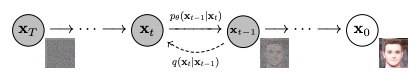 |
Training
During the training, the purpose is to learn the parameters of the diffusion kernels. Here, we will present only the case where the known distribution is gaussian. Associated formulas are given in the following table.
| Distribution and kernels | Formulas |
|---|---|
| \(\pi (\mathbf{x}^T)\) | \(\mathcal{N}\left(\mathbf{x}^{(T)} ; \mathbf{0}, \mathbf{I}\right)\) |
| \(q\left(\mathbf{x}^{(t)} \mid \mathbf{x}^{(t-1)}\right)\) | \(\mathcal{N}\left(\mathbf{x}^{(t)} ; \mathbf{x}^{(t-1)} \sqrt{1-\beta_t}, \mathbf{I} \beta_t\right)\) |
| \(p\left(\mathbf{x}^{(t-1)} \mid \mathbf{x}^{(t)}\right)\) | \(\mathcal{N}\left(\mathbf{x}^{(t-1)} ; \mathbf{f}_\mu\left(\mathbf{x}^{(t)}, t\right), \mathbf{f}_{\Sigma}\left(\mathbf{x}^{(t)}, t\right)\right)\) |
\(\mathbf{f}_\mu\left(\mathbf{x}^{(t)}, t\right)\), \(\mathbf{f}_{\Sigma}\left(\mathbf{x}^{(t)}, t\right)\) are learned. \(\beta_{1...T}\) are learned implicitly.
To learn these functions, the probability that the generative model assigns to the data is needed and is defined such as:
\[p\left(\mathbf{x}^{(0)}\right)=\int d \mathbf{x}^{(1 \cdots T)} p\left(\mathbf{x}^{(0 \cdots T)}\right)\]However, with this definition, we cannot verify that the reverse trajectory is well defined through all the markov chain. Therefore the authors reformulated \(p\left(\mathbf{x}^{(0)}\right)\) in order to make appear \(q\left(\mathbf{x}^{(t)} \mid \mathbf{x}^{(t-1)}\right)\) and \(p\left(\mathbf{x}^{(t-1)} \mid \mathbf{x}^{(t)}\right)\):
\[p\left(\mathbf{x}^{(0)}\right) = \int d \mathbf{x}^{(1 \cdots T)} q\left(\mathbf{x}^{(1 \cdots T)} \mid \mathbf{x}^{(0)}\right) p\left(\mathbf{x}^{(T)}\right) \prod_{t=1}^T \frac{p\left(\mathbf{x}^{(t-1)} \mid \mathbf{x}^{(t)}\right)}{q\left(\mathbf{x}^{(t)} \mid \mathbf{x}^{(t-1)}\right)}\]Their purpose is to maximize the model log likelihood: \(L=\int d \mathbf{x}^{(0)} q\left(\mathbf{x}^{(0)}\right) \log p\left(\mathbf{x}^{(0)}\right)\)
that can be under-estimated with:
\[K=\int d \mathbf{x}^{(0 \cdots T)} q\left(\mathbf{x}^{(0 \cdots T)}\right) \log \left[p\left(\mathbf{x}^{(T)}\right) \prod_{t=1}^T \frac{p\left(\mathbf{x}^{(t-1)} \mathbf{x}^{(t)}\right)}{q\left(\mathbf{x}^{(t)} \mathbf{x}^{(t-1)}\right)}\right]\]from which we can make the KL divergence appear:
\[K=-\sum_{t=2}^T \int d \mathbf{x}^{(0)} d \mathbf{x}^{(t)} q\left(\mathbf{x}^{(0)}, \mathbf{x}^{(t)}\right) D_{K L}\left(q\left(\mathbf{x}^{(t-1)} \mid \mathbf{x}^{(t)}, \mathbf{x}^{(0)}\right)|| p\left(\mathbf{x}^{(t-1)} \mid \mathbf{x}^{(t)}\right)\right) + C\]with \(C = H_q\left(\mathbf{x}^{(T)} \mid \mathbf{X}^{(0)}\right)-H_q\left(\mathbf{X}^{(1)} \mid \mathbf{X}^{(0)}\right)-H_p\left(\mathbf{x}^{(T)}\right)\) and \(H\) the entropy.
Multiple distributions
It is possible to combine 2 distributions. Let \(r\left(\mathbf{x}^{(0)}\right)\) be a second distribution or a bounded positive function, we have the following new distribution:
\[\tilde{p}\left(\mathbf{x}^{(0)}\right) \propto p\left(\mathbf{x}^{(0)}\right) r\left(\mathbf{x}^{(0)}\right)\]“This distribution can be treated either as a small perturbation to each step in the diffusion process, or often exactly multiplied into each diffusion step.”
Data
- Toy problems:
- swiss roll
- binary heartbeat distribution
- Images:
- MNIST
- CIFAR-10
- Dead Leaf Images
- Bark Texture Images
Results
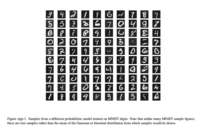


They obtain state of the art results with an elegant method.
References
-
Ho, J., Jain, A., & Abbeel, P. (2020). Denoising diffusion probabilistic models. Advances in Neural Information Processing Systems ↩