Deformable Convolutional Networks
Notes
- Code is available here: repo
Highlights
- The objective of this paper is to propose a method to adapt CNN to different geometries.
- The innovation comes from the addition of layers that learn the “stride” in order to have filters on a non-regular grid.
- The proposed method is interesting for classification, segmentation and object tracking tasks.
Introduction
For a neural network, geometric transformations, viewpoints and partial deformations are difficult to learn. Most of the time, to generalise an architecture during learning, known geometric deformations such as scaling, rotation or shearing are applied. However, there is no mechanism to help the model learn the geometric variations. This paper presents a new method capable of adapting receptive fields to understand more complex transformations. The proposed mechanism is trainable end-to-end and adaptable to any CNN-based architecture.
Method
Basic convolution and limitation
The following illustration is a simple convolution with a kernel size of \(3 \times 3\) and a stride of \(1 \times 1\). This calculation can be written as follows:
\[y(p_0) = \sum_{p_n \in R}w(p_n) \cdot x(p_0 + p_n)\]with \(p_n\) being the receptive field of the predefined convolution in the grid \(R\). In this specific case, the grid is equal to:
\[R = \{ (-1,-1), (-1, 0), (0, -1), ..., (0, 1), (1, 0), (1, 1) \}\]The grid \(R\) is static during training and inference. Thus the receptive field of classical convolution is limited. To increase it, the kernel size, the pitch or the number of cascaded convolution can be increased.
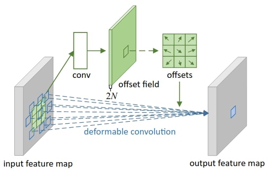
Deformable convolution
In the proposed approach, the convolution operation can be rewritten as follows:
\[y(p_0) = \sum_{p_n \in R}w(p_n) \cdot x(p_0 + p_n + \Delta p_n)\]\(\Delta p_n\) correspond to the learnable grid. For \(3 \times 3\) convolution, we have:
\[\Delta _R = \{ (\Delta {x^1}, \Delta {y^1}), (\Delta {x^2}, \Delta {y^2})), ..., (\Delta {x^9}, \Delta {y^9}) \}\]In practice, additional layers are added to learn these components. For a \(3 \times 3\) convolution, 18 additional parameters are learned. The illustration below shows the mechanism:
An interesting point is that the sampling position is adaptable to the geometric transformation, especially in the sub-images below (c,d), where scaling and rotation have been applied.

In this scenario, the sample positions do not need to be integers. For fast calculation, the bilinear interpolation is implemented as follows:
\[x(p) = \sum_q max(0,1 - |p_x - q_x| ) \cdot max(0,1 - |p_y - q_y| )\cdot x(q)\]With \(p = p_0 + p_n + \Delta p_n\).
Deformable RoI Pooling (for Region Proposal Network)
RoI pooling
The same principle can be applied to the pooling operation. Basic RoI average pooling is given by the following equation:
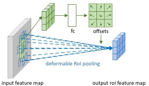
\[y(i,j) = \sum_{p \in bin(i, j)} \frac{ x(p_0 + p_n)}{n_{ij}}\]With \(bin(i,j)\) the grid surrounding the pixel at coordonate \((i,j)\), and \(n_{ij}\) the size of that grid. Just like for deformable convolution, an additional layer is added to learn the offset:
\[y(i,j) = \sum_{p \in bin(i, j)} \frac{ x(p_0 + p_n + \Delta p_{ij})}{n_{ij}}\]Illustration below shows the mechanism:
Position-Sensitive (PS) RoI Pooling
Instead of applying pooling on the input feature maps, they are converted to \(k^2\cdot (C+1)\) new feature maps, with \(k\) the size of the output, C the number of classes and +1 for the background.

The major difference can be shown in the following equation:
\[y(i,j) = \sum_{p \in bin(i, j)} \frac{ x_{ij}(p_0 + p_n + \Delta p_{ij})}{n_{ij}}\]Where \(x(i,j)\) is this time learned by the convolutional layer and depends on the class.
Experiment
Experiments were performed on different kinds of architectures and applications:
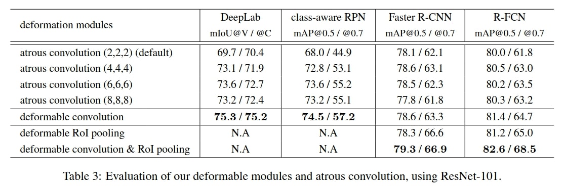
- Add Deformable ConvNets in feature extractor network (ResNet-101):
- Connect it to different networks for different applications:
- DeepLab (segmentation).
- Category-Aware (object detection - 2 classes only).
- Faster R-CNN (object detection).
Quantitative results
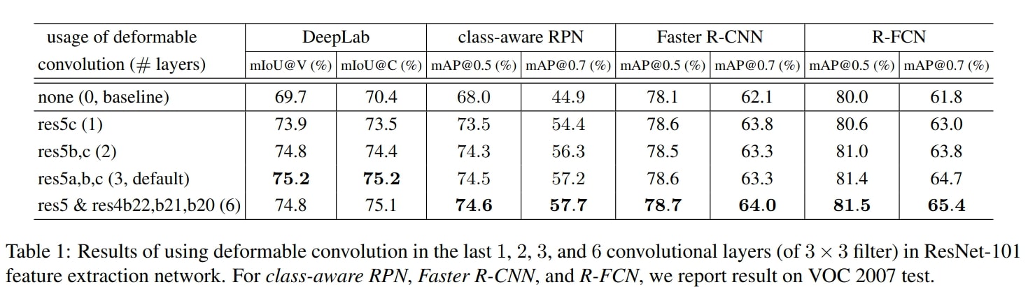
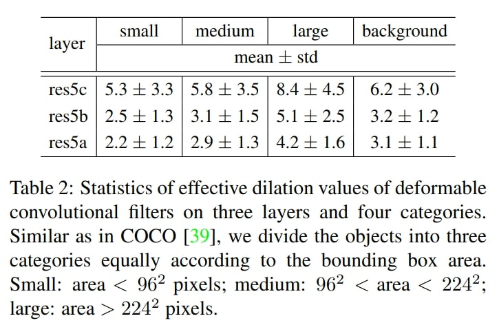
Remarks on table 2:
- The receptive field sizes of deformable filters are correlated with object sizes, indicating that the deformation is effectively learned from image content.
- The filter sizes on background regions are between those on medium and large objects, indicating that a relatively large receptive field is necessary for recognizing background regions.
Qualitative results

Conclusions
- The proposed method significantly improves the accuracy for image segmentation and object detection tasks.
- Any kind of architecture using convolution and pooling can explore the benefits of Deformable ConvNets.