Sparse Multi-Channel Variational Autoencoder for the Joint Analysis of Heterogeneous Data
Notes
- Here are some (highly) useful links: repo, video, slides
- This post has been jointly created by Olivier Bernard, Romain Deleat-Besson and Nathan Painchaud.
Highlights
- The objective of this paper is to develop a formalism called sMCVAE (sparse multi-channel VAE) to handle heterogenous data through a VAE formulation.
-
This is achieved through two major innovations:
1) Variational distributions of each channel (type of data) are constrained to a common target prior in the latent space to bring interpretability.
this can be seen as a process of alignment
2) Parsimonious latent representations are enforced by variational dropout to make the method computationally advantageous and more easily interpretable.
Method
Starting point
-
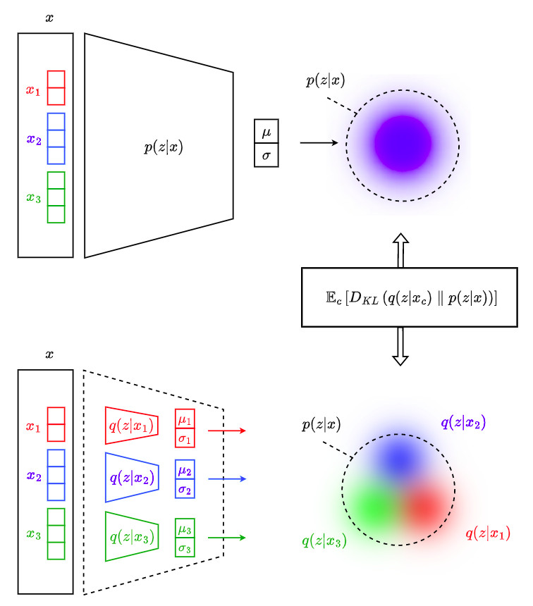
Observations (e.g. patient information) are composed by subsets of information called channels as follows:
\[\textbf{x}=\{\textbf{x}_1,\cdots,\textbf{x}_C\}\]where each \(\textbf{x}_c\) is a \(d_c\)-dimensional vector.
-
\(\textbf{z}\) is an \(l\)-dimensional latent variable which is supposed to be commonly shared by all \(\textbf{x}_c\)
-
Every channel brings by itself some information about the latent variable distribution. The posterior \(p(\textbf{z} \vert \textbf{x})\) can thus be approximated from the individual distributions \(q(\textbf{z} \vert \textbf{x}_c)\)
-
Since each channel provides a different approximation, each \(q(\textbf{z} \vert \textbf{x}_c)\) can be constrained to be as close as possible to the target posterior distribution by minimizing the following expression:
\[\mathbb{E}_{c}[D_{KL}\left( q(\textbf{z} \vert \textbf{x}_c) \parallel p(\textbf{z} \vert \textbf{x}_1,\cdots,\textbf{x}_C)\right)]\]where \(\mathbb{E}_{c}\) is the average over channels computed empirically.
The following figure illustrates the underlying concept:
Derivation of the ELBO loss
The minimization of the above equation is equivalent to the maximization of the following Evidence Lower BOund - ELBO (the corresponding demonstration is given in the appendix of this post):
\[\mathcal{L} = \mathbb{E}_{c}\left[\mathbb{E}_{\textbf{z} \sim q(\textbf{z} \vert \textbf{x}_c)}[log\left(p(\textbf{x} \vert \textbf{z})\right)] - D_{KL}\left( q(\textbf{z} \vert \textbf{x}_c) \parallel p(\textbf{z})\right) \right]\]Making the hypothesis that every channel is conditionally independent from all others given \(\textbf{z}\), we have:
\[p(\textbf{x} \vert \textbf{z})=\prod_{i=1}^{C}p(\textbf{x}_i \vert \textbf{z})\]\(\mathcal{L}\) can thus be rewritten as:
\[\mathcal{L} = \mathbb{E}_{c}\left[\mathbb{E}_{\textbf{z} \sim q(\textbf{z} \vert \textbf{x}_c)}\left[\sum_{i=1}^{C}log\left(p(\textbf{x}_i \vert \textbf{z})\right)\right] - D_{KL}\left( q(\textbf{z} \vert \textbf{x}_c) \parallel p(\textbf{z})\right) \right]\]
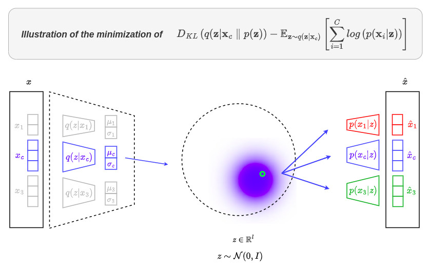
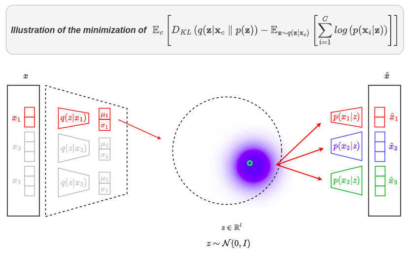
The minimization of \(\mathbb{E}_{c}[D_{KL}( q(\textbf{z} \vert \textbf{x}_c) \parallel p(\textbf{z} \vert \textbf{x}))]\) is thus equivalent to the minimization of
\[\mathcal{L^{*}} = \mathbb{E}_{c}\left[D_{KL}\left( q(\textbf{z} \vert \textbf{x}_c) \parallel p(\textbf{z})\right) - \mathbb{E}_{\textbf{z} \sim q(\textbf{z} \vert \textbf{x}_c)}\left[\sum_{i=1}^{C}log\left(p(\textbf{x}_i \vert \textbf{z})\right)\right]\right]\]The following figure illustrates the minimization of \(\mathcal{L^{*}}\):

Reconstruction of missing channels
-
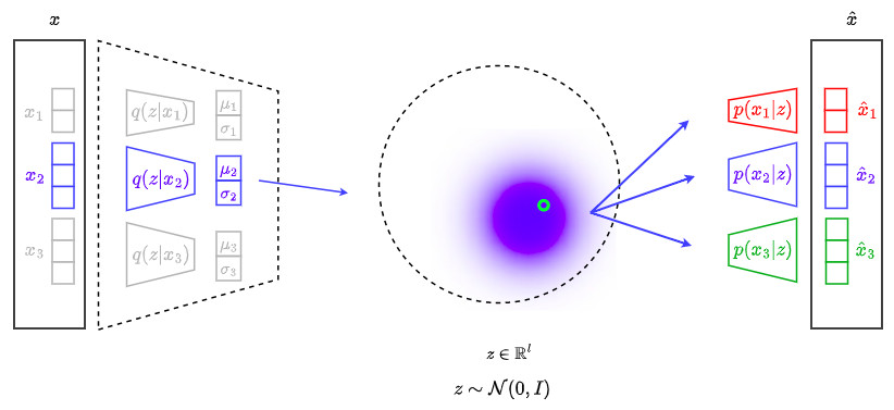
The terms \(\mathbb{E}_{\textbf{z} \sim q(\textbf{z} \vert \textbf{x}_c)}\left[\sum_{i=1}^{C}log\left(p(\textbf{x}_i \vert \textbf{z})\right)\right]\) force each channel to be able to perform the joint decoding of itself and every other channel at the same time
-
This property allows to reconstruct missing channels \(\{\hat{\textbf{x}}_i\}\) from the available ones \(\{\tilde{\textbf{x}}_j\}\) as:
\[\hat{\textbf{x}}_i = \mathbb{E}_j\left[\mathbb{E}_{\textbf{z} \sim q(\textbf{z} \vert \tilde{x}_c)}\left[\left(p(\textbf{x}_i \vert \textbf{z})\right)\right]\right]\]
Comparison with standard VAE
-
In case of \(C=1\), the proposed sMCVAE model is similar to a classical VAE.
-
sMCVAE is different from a VAE where all the channels are concatenated together, since such a VAE cannot handle missing channels.
-
sMCVAE is also different from a stack of \(C\) independent VAEs, where the \(C\) latent spaces are not related to each other in any way.
The dependence between encoding and decoding across channels stems from the joint approximation of the posterior distribution
Inducing sparse latent representation
Motivations
-
From simulations, the authors found that the lower bound \(\mathcal{L}\) generally reaches the maximum value at convergence when the number of fitted latent dimensions coincide with the true one used to generate the data
-
They also found that the performance of their method also depends on the effectiveness of the latent space dimensions chosen in relation to the application
-
The authors proposed to solve this issue by automatically inferring the number of (relevant) latent dimensions using a sparsity constraint on \(z\) thanks to the strategy described hereafter
Regularization via dropout
In the case of a basic neural network with a fully connected layer, we have a linear transformation between an input vector \(\textbf{z}\) and an output vector \(\textbf{x}\) (the non-linearity is applied to the vector \(\textbf{x}\) after the linear transformation).
With a generic linear transformation, we have \(\textbf{x} = \textbf{Gz}\). Regularization techniques are based on the multiplication (element-wise) of either \(\textbf{z}\) (dropout) or \(\textbf{G}\) (dropconnect) by a random variable (usually Bernoulli).
\[x_i = \sum_{k}^{} g_{ik}(\xi_{k} z_k) \; (dropout),\]with \(\xi_{k} \sim \mathcal{B}(1 − p)\)
It is possible to use continuous noise with the distribution \(\xi \sim \mathcal{N} (1; \; \alpha = \frac{p}{1-p})\). It is similar to Binary Dropout with dropout rate \(p\) and is called Gaussian Dropout. (Molchanov et al., 2017 ; Srivastava et al., 2014).
It is beneficial to use continuous noise instead of a discrete one because multiplying the inputs by a Gaussian noise is equivalent to applying Gaussian noise on the weights. This procedure can be used to obtain a posterior distribution over the model’s weights (Wang & Manning. 2013 ; Kingma et al., 2015).
The elements \(x_i\) are approximately Gaussian for the Lyapunov’s central limit theorem and their distributions have the form:
\[x_i \sim \mathcal{N} (\sum_{k}^{} \theta_{ik}; \alpha \sum_{k}^{} \theta^2_{ik} )\]with \(\alpha = \frac{p}{1−p}\) and \(\theta_{ik} = g_{ik}z_{k}(1 − p)\).
Variational dropout and sparsity
Posterior distributions on the encoder weights \(w\) that take the form \(w \sim \mathcal{N} (\mu; \alpha \mu^2)\) are called dropout posteriors.
If the variational posteriors on the encoder weights are dropout posteriors, Gaussian dropout arises.
The improper log-scale uniform is the only prior distribution that makes variational inference consistent with Gaussian Dropout (Kingma et al., 2015) :
\[p (ln |w|) = const \Leftrightarrow p (|w|) \propto \frac{1}{|w|}\]With this prior, the \(D_{KL}\) of the dropout posterior depends only on \(\alpha\) and can be numerically approximated (Molchanov et al., 2017):
\[D_{KL} (\mathcal{N} (w; \alpha w^2) || p (w) ) ≈ −k_1\sigma(k_2 + k_3 ln \; \alpha) + 0.5 ln(1 + \alpha^{−1}) + k_1\]where \(k_1 = 0.63576\), \(k_2 = 1.87320\), \(k_3 = 1.48695\), and \(\sigma\)(·) is the sigmoid function.
Since the optimization of \(D_{KL}\) promotes \(\alpha \to \infty\) (\(\alpha = \frac{p}{1−p}\)), the implicit drop rate \(p\) tends to 1. The associated weight \(w\) can then be discarded. Indeed, unless that weight is beneficial for the optimization objective to maximize the data log-likelihood, it will be tend towards zero. Thus, sparsity arises naturally.
Sparse Multi-Channel VAE
This part will be completed later (After the post on (Sparse) Variational Dropout).
Results
Medical imaging data
The dataset is composed of
- 504 subjects of the Alzheimer’s Disease Neuroimaging Initiative (ADNI) database
- Clinical channel is composed of six continuous variables: age, results to mini-mental state examination, adas-cog, cdr, faq tests, scholarity level
- Three imaging channels: structural MRI, functional FDG-PET, Amyloid-PET. For each modality, the average image intensity was computed across 90 brain regions mapped in the AAL atlas. This strategy produces 90 features arrays for each image. Lastly, data was centered and standardized across features.
Their sMCVAE was compared with:
- MCVAE - their model without the sparsity constraint
- iVAEs - learning of independant VAE per channel
- VAE - learning a single VAE that takes as input all the channels at once
For each model class, multi-layer architectures were tested, ranging from 1 up to 4 layers for the encoding and decoding structures, with a sigmoid activation applied to all layers but the last.
After training, the latent space for each model was used to classify neurological diseases (MCI and Dementia) by means of Linear Discriminant Analysis.
During inference, as far the sMCVAE or the MCVAE are concerned, each channel was used to compute a latent variable \(\textbf{z}_i\), and the average latent variables across channels was then used as input for the classification task
For the sparse method, they selected the subspace generated by the most relevant latent dimensions identified by variational dropout \((p<0.2)\). Thanks to that, they identified 5 optimal latent dimensions

The encoding of the test set in the latent space given by the sMCVAE model is depicted in the figure below, where the visualization is limited to the 2D subspace generated by the two most relevant dimensions
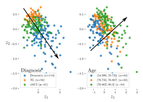
This subspace appears stratified by age and disease status, across roughly orthogonal directions.
The last figure below illustrates the capacity of the method to reconstruct plausible imaging channels when manipulating an original sample to move along interpretable trajectories in the latent space.
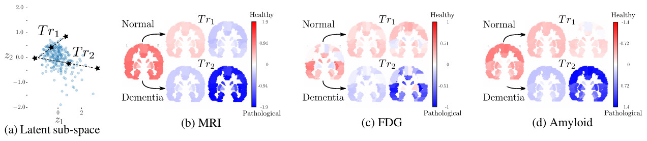
Trajectory 1 (\(T_{r1}\)) follows an aging path through the healthy subject group.
Trajectory 2 (\(T_{r2}\)) starts from the same origin as \(T_{r1}\), but follows a path were aging is entangled with a progression of the pathological factor.
Both trajectories show a plausible evolution across disease and healthy conditions
Conclusions
-
The authors proposed two innovations in this paper: i) a VAE formalism to deal with heterogeneous data structured as multi-channel; ii) the use of variational dropout to impose sparsity constraints in the latent space
-
Results are encouraging and show interesting properties of the latent space learned from a neurological application
Appendix
KL-divergence of the proposed model
\[\mathbb{E}_{c}[D_{KL}\left( q(\textbf{z} \vert \textbf{x}_c) \parallel p(\textbf{z} \vert \textbf{x}_1,\cdots,\textbf{x}_C)\right)]\] \[=\mathbb{E}_{c}[D_{KL}( q(\textbf{z} \vert \textbf{x}_c) \parallel p(\textbf{z} \vert \textbf{x}))]\] \[=\mathbb{E}_{c}\left[\int_{\textbf{z}}{q(\textbf{z} \vert \textbf{x}_c)\cdot \left[ log\left(q(\textbf{z} \vert \textbf{x}_c)\right) - log\left(p(\textbf{z} \vert \textbf{x})\right) \right] \, dz}\right]\] \[\text{using} \quad p(\textbf{z} \vert \textbf{x}) = \frac{p(\textbf{x} \vert \textbf{z}) \cdot p(\textbf{z})}{p(\textbf{x})}\] \[=\mathbb{E}_{c}\left[\int_{\textbf{z}}{q(\textbf{z} \vert \textbf{x}_c)\cdot \left[ log\left(q(\textbf{z} \vert \textbf{x}_c)\right) - log\left(p(\textbf{x} \vert \textbf{z})\right) - log\left(p(\textbf{z})\right) + log\left(p(\textbf{x})\right) \right] \, dz}\right]\] \[=\underbrace{\mathbb{E}_{c}\left[\int_{\textbf{z}}{q(\textbf{z} \vert \textbf{x}_c)\cdot log\left(p(\textbf{x})\right)\,dz}\right]}_{Eq_1} + \underbrace{\mathbb{E}_{c}\left[\int_{\textbf{z}}{q(\textbf{z} \vert \textbf{x}_c)\cdot \left[ log\left(q(\textbf{z} \vert \textbf{x}_c)\right) - log\left(p(\textbf{z})\right) \right] \, dz}\right]}_{Eq_2}-\underbrace{\mathbb{E}_{c}\left[\int_{\textbf{z}}{q(\textbf{z} \vert \textbf{x}_c)\cdot log\left(p(\textbf{x} \vert \textbf{z})\right)\,dz}\right]}_{Eq_3}\]\[Eq_1 = \mathbb{E}_{c}\left[\int_{\textbf{z}}{q(\textbf{z} \vert \textbf{x}_c)\cdot log\left(p(\textbf{x})\right)\,dz}\right]\] \[Eq_1 = \mathbb{E}_{c}[log\left(p(\textbf{x})\right)\cdot \underbrace{\int_{\textbf{z}}{q(\textbf{z} \vert \textbf{x}_c)\,dz}}_{=1}]\] \[Eq_1 = \mathbb{E}_{c}[log\left(p(\textbf{x})\right)] = log\left(p(\textbf{x})\right)\]
\[Eq_2 = \mathbb{E}_{c}\left[\int_{\textbf{z}}{q(\textbf{z} \vert \textbf{x}_c)\cdot \left[ log\left(q(\textbf{z} \vert \textbf{x}_c)\right) - log\left(p(\textbf{z})\right) \right] \, dz}\right]\] \[Eq_2 = \mathbb{E}_{c}\left[D_{KL}\left( q(\textbf{z} \vert \textbf{x}_c) \parallel p(\textbf{z})\right)\right]\]
\[Eq_3 = \mathbb{E}_{c}\left[\int_{\textbf{z}}{q(\textbf{z} \vert \textbf{x}_c)\cdot log\left(p(\textbf{x} \vert \textbf{z})\right)\,dz}\right]\] \[Eq_3 = \mathbb{E}_{c}\left[ \mathbb{E}_{\textbf{z} \sim q(\textbf{z} \vert \textbf{x}_c)}[log\left(p(\textbf{x} \vert \textbf{z})\right)] \right]\]
We finally have:
\[\mathbb{E}_{c}[D_{KL}( q(\textbf{z} \vert \textbf{x}_c) \parallel p(\textbf{z} \vert \textbf{x}))] =\] \[log\left(p(\textbf{x})\right) + \mathbb{E}_{c}\left[D_{KL}\left( q(\textbf{z} \vert \textbf{x}_c) \parallel p(\textbf{z})\right) - \mathbb{E}_{\textbf{z} \sim q(\textbf{z} \vert \textbf{x}_c)}[log\left(p(\textbf{x} \vert \textbf{z})\right)] \right]\]
This last equation can be rewritten as:
\[\mathbb{E}_{c}[D_{KL}( q(\textbf{z} \vert \textbf{x}_c) \parallel p(\textbf{z} \vert \textbf{x}))] + \mathcal{L}= log\left(p(\textbf{x})\right)\]where \(\mathcal{L}\) is the Evidence Lower BOund (ELBO), whose expression is given by:
\[\mathcal{L} = \mathbb{E}_{c}\left[\mathbb{E}_{\textbf{z} \sim q(\textbf{z} \vert \textbf{x}_c)}[log\left(p(\textbf{x} \vert \textbf{z})\right)] - D_{KL}\left( q(\textbf{z} \vert \textbf{x}_c) \parallel p(\textbf{z})\right) \right]\]
Since \(D_{KL}\) is a measure of distance between two distributions, its value is \(\geq 0\), which leads to the following relation:
\[\underbrace{\mathbb{E}_{c}[D_{KL}( q(\textbf{z} \vert \textbf{x}_c) \parallel p(\textbf{z} \vert \textbf{x}))]}_{\geq 0} + \underbrace{\mathcal{L}}_{\leq 0} = \underbrace{log\left(p(\textbf{x})\right)}_{\leq 0\text{ and fixed}}\]Thus, by tweaking \(\{q(\textbf{z} \vert \textbf{x}_c)\}_{c=1:C}\), we can seek to maximize the ELBO \(\mathcal{L}\), which will imply the minimization of the KL divergence
So the minimization of \(\mathbb{E}_{c}[D_{KL}( q(\textbf{z} \vert \textbf{x}_c) \parallel p(\textbf{z} \vert \textbf{x}))]\) is equivalent to the maximization of \(\mathcal{L}\), or the minimization of
\[\mathcal{L^{*}} = \mathbb{E}_{c}\left[D_{KL}\left( q(\textbf{z} \vert \textbf{x}_c) \parallel p(\textbf{z})\right) - \mathbb{E}_{\textbf{z} \sim q(\textbf{z} \vert \textbf{x}_c)}[log\left(p(\textbf{x} \vert \textbf{z})\right)]\right]\]