What is being transferred in transfer learning?
Context
In cases where we lack a large amount of data or we want a fast training, we are interested in pre-trained networks that can generalize well from a source domain to a target domain.
Transfer learning consists in training a model on source data and then fine-tune it on the target data, and has encountered a big success in several applications. Still, it is not clear:
- What is needed for a successful transfer leaning?
- Which parts of the network make transfer learning work?
In this paper, the authors try to answer to these questions. Their code is available here.
Experimental Setup
Pre-trained and randomly initialized models are investigated in the image classification setting.
- Data:
- Source data for pre-training: ImageNet.
- Target data for downstream tasks: CheXpert (X-ray) and DomainNet (real, clipart and quickdraw).
- Models:
- Architecture: ResNet-50.
- P-T: pre-trained model then fine-tuned on the target domain.
- RI-T: random initialization model trained on the target domain.
Experiments
1. Role of feature reuse in transfer learning
Intuition: reusing the pre-trained feature hierarchy explains the success of transfer learning. Therefore, we expect better performances when doing transfer learning on target domains that share similar visual features with the source domain.

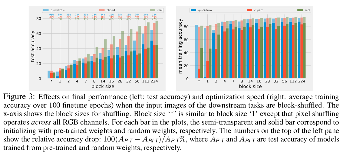
However, even distant target domains present enhanced performances with transfer learning. Are some other factors other than feature reuse being useful for the target domain? To check this, they progressively destroy high level visual features on target images and evaluate the performance loss.


Conclusion:
- Feature reuse is paramount in transfer learning.
- Low-level statistics also boost the performance of transfer learning and in particular training speed.
2. What are the differences between P-T and RI-T models?
By looking at the mistakes made by each model:
- Samples for which P-T is incorrect and RI-T is correct are mostly ambiguous samples.
- Samples for which P-T is correct and RI-T is incorrect are mostly non-ambiguous samples.
- 2 P-T models make very similar mistakes, whereas 2 RI-T models make more diverse mistakes.
How similar are two P-T models in the feature space?
Center Kernel Alignment is used as the similarity index (Kornblith at al (2019) [1]).

What is the distance of the models in the parameter space?

Conclusion:
- Model initialization has a big impact in feature similarity.
- P-T models are reusing the same features and are close to each other compared to RI-T models.
3. Generalization performance of P-T and RI-T models
“A commonly used criterion for better generalization performance is the flatness of the basin of the loss landscape near the final solution. In a flat basin, the weights could be locally perturbed without hurting the performance, while in a narrow basin, moving away from the minimizer would quickly hit a barrier, indicated by a sudden increase in the loss.”
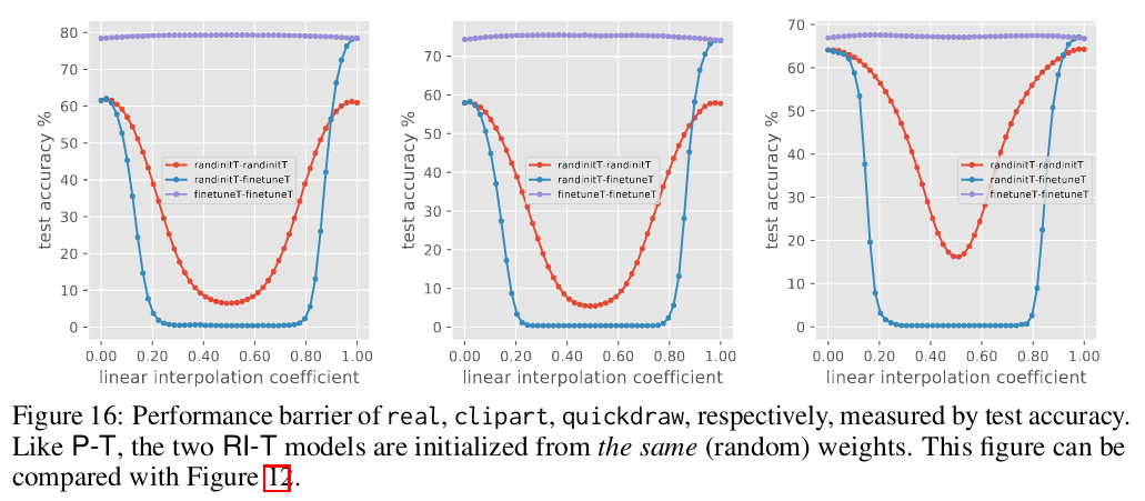
Let \(\Theta_1\) and \(\Theta_2\) be the weights corresponding to 2 different solutions. We can create a low-loss path between them by defining a set of models from the interpolation of the two set of weights: \(\{\Theta_{\lambda} = (1-\lambda)\Theta_1 + \lambda\Theta_2\}.\)
Garipov et al (2018) [2] saw that two solutions can be connected via a non-linear low-loss path. Performance barriers occur in this path unless the two solutions are in the same flat basin of the loss landscape.

Conclusion:
- There is no performance barrier between P-T models: “pre-trained weights guide the optimization to a flat basin of the loss landscape”.
- RI-T models present a performance barrier, even with equal random initializations: they are in different basins of the loss landscape.
- P-T models have better generalization capacities.
4. Where is feature reuse happening?
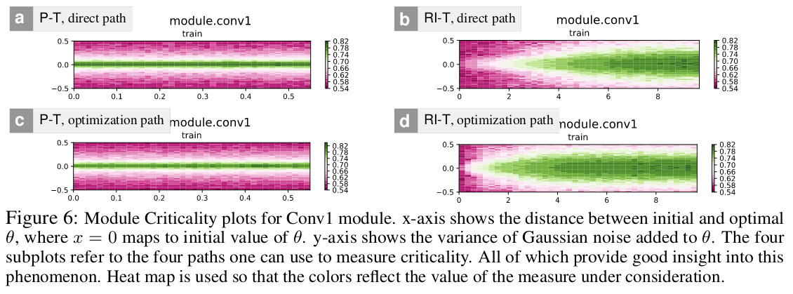
Zhang et al (2019) [3] saw experimentally that some layers of a network are less robust to perturbation than others, and are therefore more critical. Module criticality can be measured by rewinding the module values back to their initial value while keeping the other trained values fixed, and test the model performance.

Criticality of a module can also be measured by looking at the model performance in the path connecting the first and final value of a module weights during training while keeping the other modules at their final values, and then measuring the width of the valley formed by this path.

Conclusion:
- For fine-tuned models, deeper layers are more critical than lower layers. This means that lower layers are responsible for more common features and deeper layers are responsible for more task-specific features.
5. Which pre-trained checkpoint model to use?
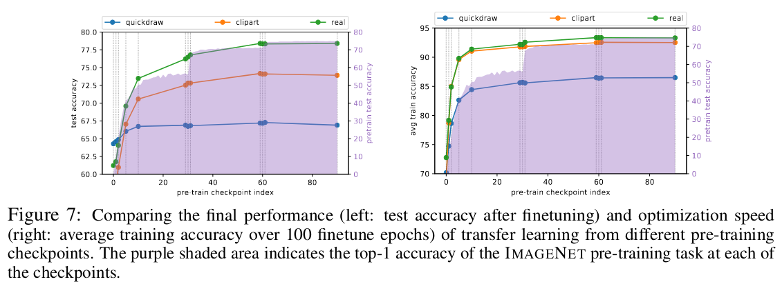
The standard practice is to take the checkpoint giving the best performance on the source data, or the last one. But the performance on source data may not be directly linked to the performance in target data.

Conclusion:
- We can use earlier checkpoints corresponding to the beggining of the last plateau in the source task instead of the last checkpoint. This corresponds to the time when the pre-trained model is entering its final basin.
- In Abnar et al (2022) [4], the same authors see across many experiments that: “as we increase the upstream accuracy, performance of downstream tasks saturate”.
Conclusions
- The authors use a wide range of tools for the analysis and understanding of models.
- Both image features and low-level statistics play a role in the good performance of transfer learning on target tasks.
- Fine-tuned models are close to each other in the parameter and feature space.
- Fine-tuned models have better generalization capacities than randomly initiliazed models.
- We can use earlier checkpoint models of the pre-trained model and this will not decrease the fine-tuning performance.