Fixing bias in reconstruction-based anomaly detection with Lipschitz discriminators
Context
(For more context, see the post about VT-ADL)
- Anomaly detection, also called outlier detection, one-class classification and many other terms, is the process of detecting events/items that deviate significantly from the normality. A distribution of the normal class is estimated and the event/item is said to be anomalous if it does not belong to this distribution.
- Here we tackle the problem of anomaly detection in images in the context of machine learning, meaning we will train a network (or another kind of algorithm) on normal images only, and then, at inference, we will try to classify images as normal VS anomalous.
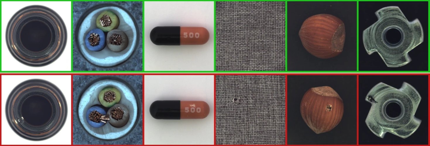
Example of normal (green) VS anomalous (red) image on the well known MVTecAD dataset - More formally : the objective is to estimate the probability density (or at least its support) in a high dimensional space, the image space. Auto-encoders have proven useful in this task because of their ability to reduce the dimensionality of the problem.
- The objective of this paper is to propose a new anomaly detection method which uses Lipschitz constrained discriminators, to compare the performances to auto-encoder based methods and analyse failure cases.
Highlights
- Introduction of new outlier detection network based on Lipschitz discriminator
- Comparison with other outlier detection methods on MNIST, CIFAR 10.
- Analysis of the failure of Auto-Encoder based outlier detection methods.
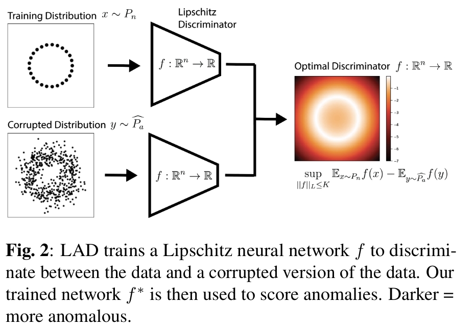
Proposed method : Lipschitz anomaly disccriminator (LAD)
\[L = \mathbb{E}_{x \sim P_n} [f(x)] - \mathbb{E}_{x \sim \hat{P_a}} [f(x)] + \lambda \mathbb{E}_{x \sim P_x} [(||\nabla_x f(x)||_2 - 1)^2]\]Where \(P_n\) is the normal distribution and \(\hat{P_a}\) is supposed to model the “true anomaly distribution” \(P_a\). In this paper, \(\hat{P_a}\) is a corrupted version of \(P_n\). Samples from \(\hat{P_a}\) could have been generated through a generator (like in GANs) but the authors reported better performances with a simple corruption process.
\(\mathbb{E}_{x \sim P_n} [f(x)]\) will maximize the probability that the discriminator attributes high scores to normal samples and \(- \mathbb{E}_{x \sim \hat{P_a}} [f(x)]\) will maximize the probability that the discriminator attributes low scores to corrupted samples.
The last term \(\mathbb{E}_{x \sim P_x} [(||\nabla_x f(x)||_2 - 1)^2]\) ensures that the network function \(f\) is 1-Lipschitz. (needs a little bit more mathematical investigation but :) the Wasserstein-1 metric \(\mathbb{E}_{x \sim P_n} [f(x)] - \mathbb{E}_{x \sim \hat{P_a}} [f(x)] + \lambda \mathbb{E}_{x \sim P_x}\) could not be achieved if the network was not 1-Lipschitz. \(P_x\) is obtained as a linear interpolation between \(P_n\) and \(\hat{P_a}\).
Advantages : mathematically sound (some proofs are given in the paper), make use of the well known Wasserstein-1 metric.
Drawback: need for an arbitrary corruption process, as the autors said “The choice of the anomaly distribution to train against is important and useful in building inductive bias into the model”.
The authors, as a response to this obvious drawback, say that “Existing models implicitly build in an assumption on the anomaly distribution. For example, overparameterized autoencoders assume points are far from the span of the data”
Experimental evaluation
The authors propose two experiments that I will describe bellow.
1) Training set contamination
The authors propose to evaluate their model performance’s with a classic easy anomaly detection task on MNIST : assuming one digit is the normal class and the others are anomaly (e.g. \(P_n\) is a set of “3” and \(P_a\) are “1”, “4”, etc.).
They then add training set contamination (e.g. “5” in the training set when the normal class is “3”) from 0% to 10%, compare to other SOTA methods and demonstrate the superiority of their method LAD (Table 1 with contamination fraction on top).
They also show superiority of their method when combined to a Convolutional Auto-Encoder (LAD + CAE).
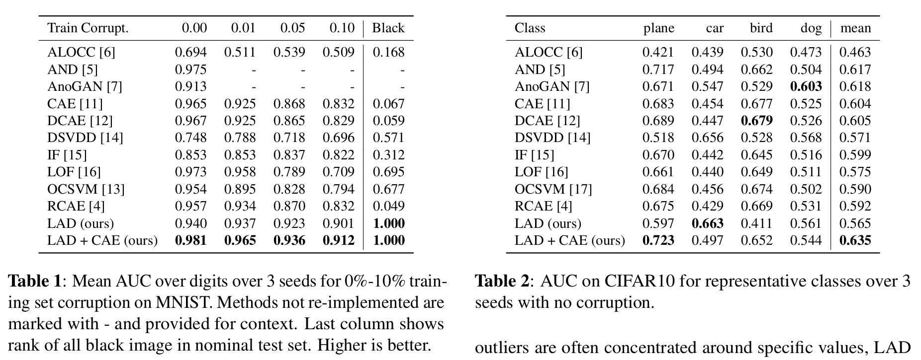
An impressive result is that the corruption process (\(P_n\) to \(\hat{P_a}\)) used here on MNIST is patch shuffling (with 4x4 patches), which is very far from the true anomaly distribution \(P_a\). (e.g. an image of a “3” shuffled will look very different from an image of a “4”). While \(\hat{P_a}\) is very different from \(P_a\), the results are competitive.
2) Bias towards interpolated points
The authors pointed out that the inductive bias from an Auto-Encoder reconstruction error was that the anomalies will be far from the mean of the training data in the latent space. They propose to investigate this bias in an experiment.
Black image in MNIST
They first show every anomaly detection method the “all black image”. The all black image is very abnormal because it is not a digit, but very easy to reconstruct for an Auto-Encoder because it has learn to reconstruct black part of images. Result of the anomaly score for each method are shown in table 1 (represented by the ranking of the image, from 0 to 1 with 1 being ranked first).
Reconstructions based methods are CAE, DCAE, RCAE, AND, ALOCC and AnoGAN, SVM based methods are OCSVM and DSVDD and other machine learning methods IF and LOF.
Mean image in CIFAR-10
When training on CIFAR-10 (normal class is one of the class and anomalies are other classes, like in MNIST), they find out that the performances vary greatly among classes (table 2).
They explain this by looking at the mean image for each class : in class such as birds, the samples are usually close to the mean image, whereas in cars for instance, images can be very far from the mean image (when with white background for example). This is also shown in table 2 where they give the rank of the mean image.
To showcase this even more, they display the top 100 “most normal” images in the test set when trained on cars in figure 4. We see that the LAD has images that are far from the mean (i.e. with clear background), and that it mistakes trucks for cars, but not animals for cars as the reconstruction based method.

Conclusion
The authors present a new method based on Lipschitz discriminators (LAD). It has the advantages of being mathematically based on “nice” properties, and make use of the well known Wasserstein-1 distance and discriminator from GANs. They present two experiments which showcase the competitivity of their method and the bias toward mean points in reconstruction-based methods.