NeRF: Representing Scenes as Neural Radiance Fields for View Synthesis
Notes
- Link to code, full paper and more examples in the project page
Highlights
- The objective of the paper is to synthesize novel views of complex 3D scenes.
- The authors use a MLP to optimize a continuous volumetric scene function on a set of 2D input views.
Introduction
What do we mean by scene function?
There are different ways to represent 3D objects or scenes: it could be a voxel representation, which is a 3D grid that represents the object. It could also be a point cloud, or a mesh. Here the authors propose to represent a scene (or 3D object) as a function. The function completely defines the object, and is learned by a MLP network.
To put it simply: one network = one function to optimize = one object
What is view synthesis in this context?
The network is optimized on a set of 2D input views: they are “pictures” of the object/ scene taken from a certain angle. From the learned function, which represents the object, one can choose a novel view, from a different angle and take a “picture” of the object from this angle. Therefore, one can then take as many pictures of the object as they want, from any angle, because the whole object is represented by the MLP.
Method
Neural Radiance Fields
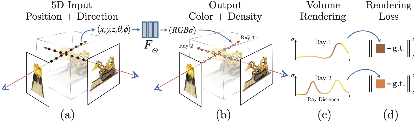
Figure 1: pipeline proposed by the authors
For one input image, the authors consider a virtual camera that takes the picture of the view. There is a ray that can be defined that stems from this camera and that passes through the object. Along this ray, points are sampled. The position, or coordinates, of these points, as well as the direction from which the ray starts are known and are used as input to the network.
For each point sampled, the network outputs its RGB color and its density, which is high when the point belongs to an object, and low when the point was sampled in an empty area.
During inference, a camera is located at a new angle, and a new set of points is sampled and from this, a new picture of the object is taken.
Architecture-wise: one MLP network with 8 fully-connected layers is learned for each scene. This MLP learns to map a position \(\boldsymbol{x}\) and a direction \(\boldsymbol{d}\) to a density \(\sigma\) and color values \(RGB\) : \(F_\Theta : (\boldsymbol{x},\boldsymbol{d}) \rightarrow (RGB,\sigma)\)
Volume rendering
In order to have the ground truth color and density values corresponding to the sampled points, standard image rendering techniques are used. These techniques will not be developped here, and are very specific to the field.
Optimizing NeRF
Positional encoding
The resconstructed scenes can be blurry in areas with complex details.
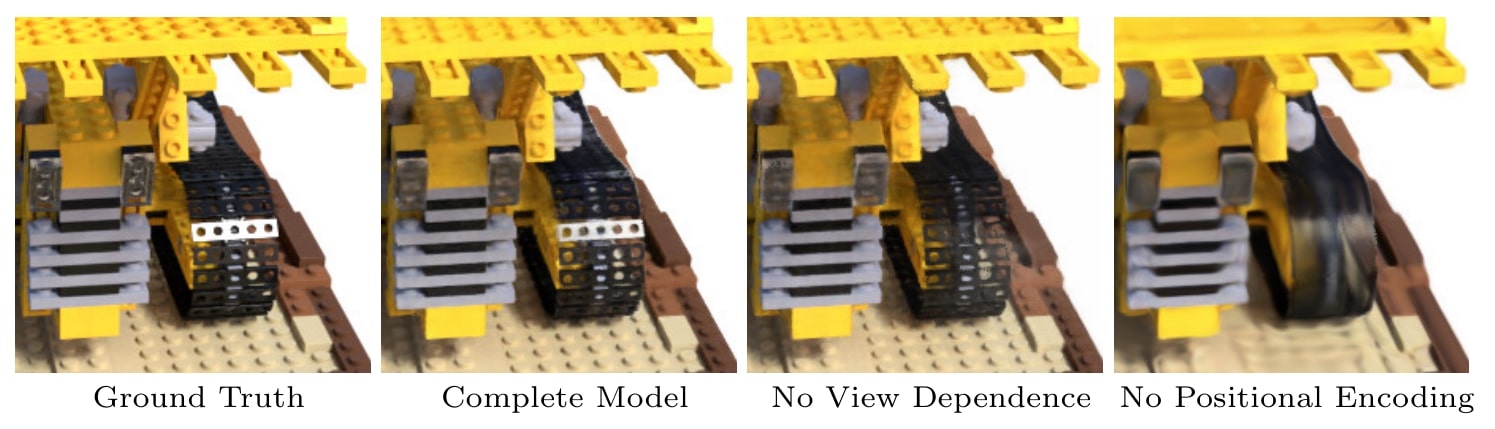
Figure 2: Visualization of the effect of positional encoding
The inputs are mapped to a higher dimensional space by using high frequency functions before being fed to the network: \(\gamma(p) = (\sin(2^{0}\pi p),\cos(2^{0}\pi p), ... ,\sin(2^{L-1}\pi p),\cos(2^{L-1}\pi p) )\).
This enables the learning of higher frequencies variations in the object.
Hierarchical sampling
Instead of sampling regularly along a camera ray, and in order to avoid uselessly sampling a lot of free space, two networks are trained.
A first “coarse” network is trained on a widely spaced set of points. This gives information about the density in certain area of the the space. Then the “fine” network is trained on points sampled on areas that are expected to contain more visible content.
This enables a more efficient sampling of the space.
Implementation
Gradient descent is used to optimize the model.
The loss used is : \(\mathcal{L} = \sum_{r\in \mathcal{R}} [ \|\hat{C}_c(\boldsymbol{r}) - C(\boldsymbol{r}) \|_{2}^{2} + \|\hat{C}_f(\boldsymbol{r}) - C(\boldsymbol{r}) \|_{2}^{2}]\)
with \(\mathcal{R}\) the set of rays in each batch, \(C(\boldsymbol{r})\), \(\hat{C}_c(\boldsymbol{r})\) and \(\hat{C}_f(\boldsymbol{r})\) the RGB colors for ground truth, coarse and fine volume predicted.
Note that the density does not appear in this loss, it is used to compute the RGB colors.
Results
This method can be used on real word or synthetic scenes. A comparison is done with three networks based on deep learning techniques.
The test is done on 2D output views of the network.
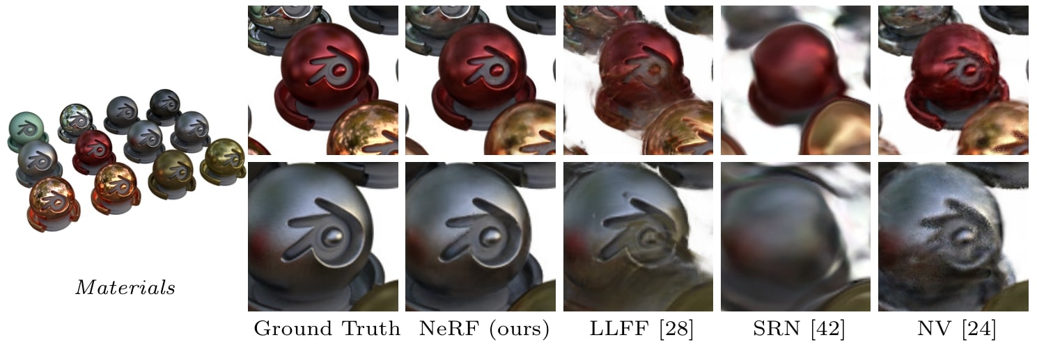
Figure 3: results on a synthetic dataset
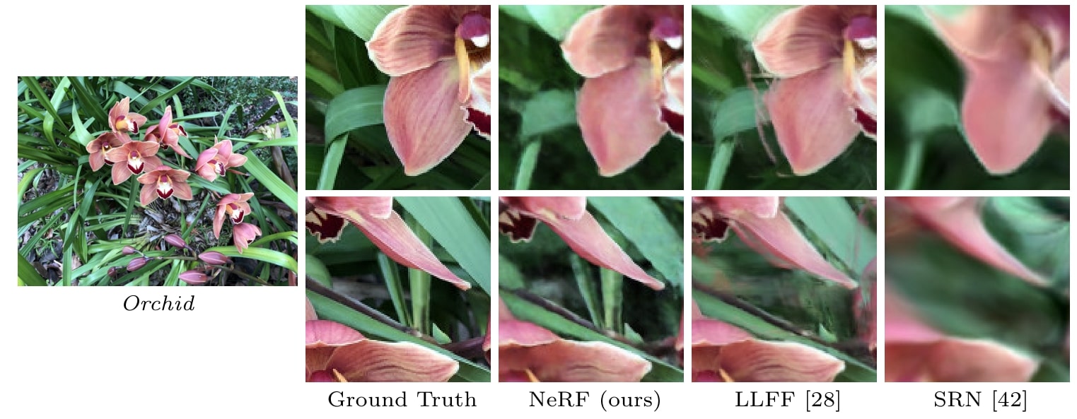
Figure 4: results on a real-world dataset
Quatitatively, the results also achieve more satisfying results than state-of-the-art, using metrics that evaluate the output 2D views.
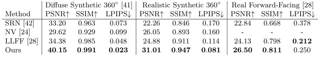
Table 1: quantitative comparaison with state-of-the-art method [metrics: SNR/SSIM (higher is better), LPIPS (lower is better))
Another advatage of this method is that, once trained, the network is lighter than the set of input images used for training. This makes it useful to overcome the issue of storage problem implied by the use voxelized representation of complex scenes.
Conclusion
- Scenes can be represented by a MLP taking position and view angle as input and outputting color and density: this is the nature of Neural Radiance Fields intrduced by this paper
- The renderings are better with the method proposed than with state-of-the-art, and has become a pilar in the field