Complementing Brightness Constancy with Deep Networks for Optical Flow Prediction
Notes
- Code is available on GitHub: https://github.com/vincent-leguen/COMBO.
Highlights
- Introduce a novel deep-learning-based optical flow estimation that can be trained in both supervised and semi-supervised manner;
- Exploit the brightness constancy (BC) model used in traditional methods;
- Decompose the flow into the physical prior and the data-driven component + uncertainty quantification of the BC model.
Introduction
What is optical flow estimation?
- Computation of the per-pixel motion between video frames.
Where can optical flow estimation be applied?
- Video compression, image registration, object tracking, etc.
Traditional methods use the brightness constancy (BC) model, which assumes the intensity of pixels is conserved during the motion. Given a random pixel \(x\), \(I_{t-1}(x) = I_{t}(x+w)\), where \(w\) is the motion of the pixel. If only small motions are considered, this constraint can be linearized to a partial differential equation and solved by variational methods:
\[\frac{\partial I}{\partial t}(t, x) + w(t, x)\cdot \nabla I(t,x) = 0\]Downsides of the BC model:
- only a coarse approximation of reality
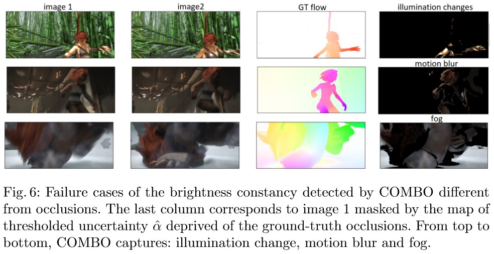
- violated in many situations: presence of occlusions, local illumination changes, complex situations such as fog
- need to inject some prior knowledge of the flow, e.g. spatial smoothness
Deep-learning-based methods can potentially solve these problems, especially considering SOTA flow estimation methods are supervised models. However, flow labeling on real images is expensive. Therefore, the training of these models has often relied on complex curriculum training on synthetic datasets and then fine-tuning to real world datasets. Recently, unsupervised approaches have been proposed that adapt the main idea of the traditional methods by adding regularization losses.
The authors propose a hybrid model that decomposes the flow estimation process into a physical flow based on the simplified BC hypothesis and a data-driven augmentation to compensate the limitations of the BC model.
Methods
Architecture

To extract the features and to estimate the physical flow, \(\hat{w}_p\), augmentation flow, \(\hat{w}_a\), and uncertaincy map, \(\hat{\alpha}\), RAFT1 architecture is used:
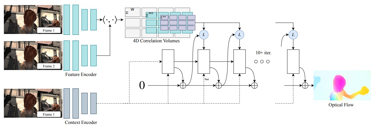
Main ideas of RAFT
- Feature encoder, \(g_\theta: \mathbb{R}^{H \times W \times 3} \rightarrow \mathbb{R}^{\frac{H}{8} \times \frac{W}{8} \times D}\):
- Extract features from image \(t-1\) and \(t\) using a simple encoder.
- Context encoder, \(h_\theta: \mathbb{R}^{H \times W \times 3} \rightarrow \mathbb{R}^{\frac{H}{8} \times \frac{W}{8} \times D}\):
- Extract context features from image \(t-1\).
- Visual similarity:
- Compute correlation between features extracted from image \(t-1\) and \(t\). \(<g_\theta(I_{t-1}), g_\theta(I_{t})> \in \mathbb{R}^{\frac{H}{8} \times \frac{W}{8} \times \frac{H}{8} \times \frac{W}{8}}\)
- Output a 4D correlation volume.
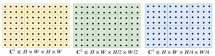
- Construct a 4-layer correlation pyramid by pooling the last two dimensions of the correlation volume.
- Give information about small and large displacements.
- Iterative updates using Gated recurrent units (GRUs):
- Current flow estimate, \(f_k\) (Initialized as 0)
- Apply the flow and update the coordinates of each pixel
- Retrieve the correlation features from the correlation pyramids:
- For each predicted pixel in \(I_t\), define a local grid of \(9\times9\) using a radius of \(4\).
- Retrieve the correlations within this neighborhood for each pyramid level to obtain the information about small and large movements.
- Concatenate the retrieved correlation features of each level \(\in \mathbb{R}^{\frac{H}{8} \times \frac{W}{8} \times 9 \times 9 \times 4}\)
- Inject the concatenation of flow, correlation, and context features to the GRU
- Predict flow update, \(\Delta f\)
- Update the flow estimate, \(f_k = f_k + \Delta f\)
- Upsample the predicted flow since the output flow is computed at 1/8 resolution.
Innovations
Instead of predicting only the physical flow \(\hat{w}_p\) using GRUs, the authors use another GRU block to predict the augmentation flow and uncertainty map.
The final flow is given as: \(\hat{w}(x) = (1- \hat{\alpha}(x))\hat{w}_p(x) + \hat{\alpha}\hat{w}_a(x)\). Similarly, the ground truth flow is decomposed as: \(w^*(x) = (1- \alpha^*(x))w_p^*(x) + \alpha^*w_a^*(x)\). However, this decomposition is not necessarily unique. Hence, the following constraints are used during the optimization:
\[\begin{equation} \min_\limits{w_p, w_a} ||(w_a, w_p)|| \text{subject to}\\ \begin{cases} (1-\alpha^*(x))w_p(x) + \alpha^*(x)w_a(x) = w^*(x) & (1)\\ (1-\alpha^*(x))|I_{t-1}(x)-I_{t}(x+w_p(x))| = 0 & (2)\\ \alpha^*(x) = \sigma(|I_{t-1}(x)-I_{t}(x+w^*(x))|) & (3)\\ \end{cases} \end{equation}\]- (1): Flow decomposition
- (2): BC flow constraint = \(\vert I_{t-1}(x)-I_{t}(x+w_p(x))\vert\), weighted by \((1-\alpha^*(x))\) as this is an unsupervised loss and is not always verified.
- (3): Compensation in case of violation of the BC. \(\sigma(\cdot)\) nonlinear function \(\rightarrow [0,1]\). If \(\alpha^*(x) = 0\), the BC assumption is verified. If not, compensation via \(\hat{w}_a\)
Training loss:
\(\mathcal{L}(D, \theta) = \underbrace{\lambda_p \|\hat{w}_p-w^*_p\|^2_2 + \lambda_a\|\hat{w}_a-w^*_a\|^2_2 + \lambda_{total}\|\hat{w}-w^*\|^2_2}_{\text{supervised loss}} + \underbrace{\lambda_{photo}\mathcal{L}_{photo}(D,\theta)}_{\text{unsupervised loss}} + \underbrace{\lambda_w\|(\hat{w}_a, \hat{w}_p)\|^2_2}_{\text{regularization}} + \underbrace{\lambda_\alpha\mathcal{L}_\alpha(D,\theta)}_{\text{uncertainty loss}}\),
- \(D:\) supervised or unsupervised image pairs
- \(\mathcal{L}_{photo}(D,\theta):\) \((1-\alpha^*(x))\vert I_{t-1}(x)-I_{t}(x+w_p(x))\vert_1\)
- \(\|(\hat{w}_a, \hat{w}_p)\|^2_2:\) minimization of the norm of the concatenation of \((\hat{w}_a, \hat{w}_p)\) vector. (Prevent degenerate cases and allow compensation with minimal correction \(\|\hat{w}_a\|\))
- \(\mathcal{L}_\alpha(D,\theta):\) \(\| \alpha^*(x) - \sigma(\vert I_{t-1}(x)-I_{t}(x+w_p(x))\vert_1) \|^2_2\)
Training strategy:
- Curriculum learning: Use of the ground truth \(\alpha^*\) with high probability at the beginning and decrease progessively this probability towards 0 to rely more and more on the prediction \(\hat{\alpha}\).
- Supervised learning: Only use labeled image pairs.
- Semi-supervised learning: Mix labeled and unlabeled image pairs in a mini-batch. For labeled data, minimize the full training loss. For unlabeled data, only minimize unsupervised loss and block the gradient flow in the uncertainty branch \(\alpha\) since \(\alpha\) can only be estimated in supervised mode. This means setting \(\lambda_{photo}=1\) and \(\lambda_p=\lambda_a=\lambda_{total}=\lambda_w=\lambda_\alpha=0\). In the unsupervised mode, the curriculum learning is not applied.
Benchmarking datasets
The authors benchmarked COMBO on 3 datasets: FlyingChairs, MPI Sintel and KITTI-2015 in supervised and semi-supervised contexts.
Results
Supervised results
The authors pretrained their model on FlyingChairs (C) and FlyingThings (T). They then fintune on Sintel (S) by combining data from Sintel, KITTI-2015 (K), and HD1K (H). The table below shows that COMBO outperforms RAFT on three training stages, demonstrating the usefulness of the augmentation model.

The authors then evaluate the generalizability of their model by comparing it to other SOTA networks.

Semi-supervised results
The authors also report the results obtained using semi-supervised fine-tuning from FlyingChairs or Sintel checkpoints. Surprisingly, the semi-supervised trained COMBO outperforms the supervised-trained COMBO and RAFT.
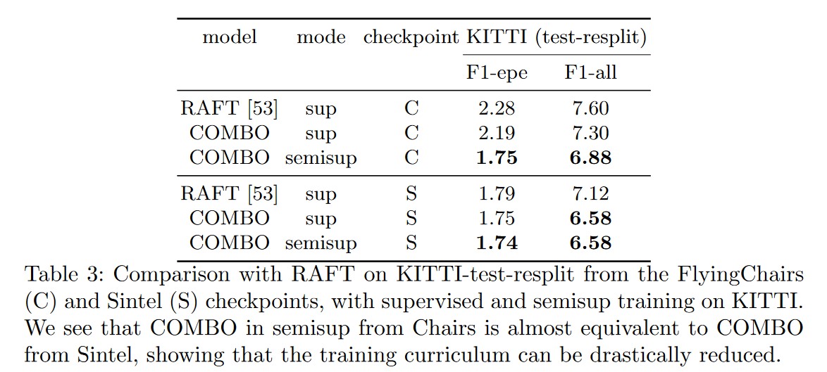
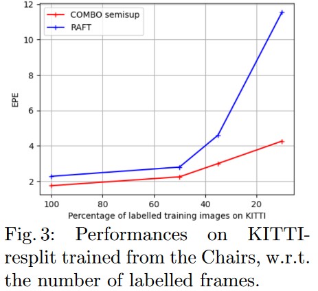
When reducing the number of labeled frames on KITTI-resplit, they observe a slower degradation of results as compared to RAFT.
Predictions

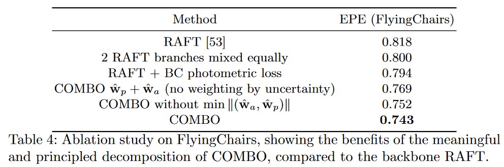
Ablation study
Conclusions
The authors introduced COMBO, a new physically-constrained architecture for optical flow estimation. The novel combination of supervised and unsupervised loss allows COMBO to achieve SOTA results on several benchmarks. Finally, the semi-supervised learning scheme further improves the performance and greatly simplifies the training curriculum.