A ConvNet for the 2020s
Highlights
- ConvNeXt is a new fully convolutionnal architecture that aim to be a generic backbone for computer vision tasks.
- It achieved state-of-the-art performances on several classic tasks, surpassing Hierarchical Transformers such as Swin.
- It has been built from the vanilla ResNet-50 network by incrementally addind design choices inspired from Transformers or other ConvNets.
- All ConvNeXt models, including pre-trained weights, are available on the GitHub of the project.
Introduction
A brief history of deep learning for computer vision
The 2010s was marked by the stricking arrival of deep learning for many tasks. In computer vision, the revolution came from convolutional neural networks, that quickly impose themselves of the go-to models for computer vision. Since the introduction of AlexNet in 2012, many other refined architectures such as VGGNet, ResNet, EfficientNet and all their derivatives have used the principle of learnable convolution to achieve increasingly good performances in image classification, segmentation, object detection, etc. The sliding window strategy and the inductive biases (translation equivariance, pattern recognition, spatial local information, etc.) that it introduces are intruitively adapted to visual processing. Hence, convolution networks have been proved to be very effective for many computer vision tasks.
On an other side of deep learning’s applications, natural language processing (NLP) have also kwnown their own revolution with the introduction of Transformers in 2017. Based on the principle of computation of attention between tokens, it progressively the recurrent neural networks that were used before.
In 2020, Alexey Dosovitskiy and his team bridged the gap between the two domains by introducing the Vision Transformer (ViT). The promise of the network was to be able to compute global attention between every regions of an image – gather local information of the into patches – without introducing any image-specific inductive biases. The network outperformed ResNet-like models by a significant margin on image classification tasks. Howerver, their was still some issues with it, two of them being that it has a quadratic space and time complexity and that it may not be as performant when used for other computer vision tasks, such as segmentation, where the sliding-windows paradigm seem even more important.
The next major breakthrough came with the Swin Transformer, a hierarchical Transformer that achieved state-of-the-art performances on several classic tasks and showed for the first time that Transformers can be employed as generic backbone in computer vision. It introduced alterned shifting windows in order to focus attention computation on local tokens and increase progressively their receptive field, also allowing to reduce the space and time complexity to linear.
Motivation
Even though the dominance of Transformers-based architectures can sometimes be attributed to the inheret superiority of the multi-head self-attention mechanism, the Swin Transformer also reveal that essence of the convolution has not become irrelevant. In the end, Swin Transformer is a step closer to ConvNets that the original ViT was, and ConvNets and Swin Transformer are different and similar at the same time. They both introduce inductive biases to capture the information on images, but their training procedure and macro and micro level architecture design are quite different.
While Vision Transformers were a paradigm shift, ConvNets themselves evolved mostly incrementally for a decade. The design improvements that have been explored since 2012 have been researched separately, but no study tried to sum up all of them into a ‘ResNet 2.0’. The goal of the authors with this paper is to investigate the architectural distinctions between ConvNets and Transformers and modernize ConvNets to see what performances a purely convolutional network that integrates recent architecture designs can achieve.
Methodology
The authors starts from the vanilla ResNet50 and ResNet200 models (shown in Fig. 1) and changed them step by step by integrating or not many design choices. These two models are respectively comparable in terms of FLOPs and number of parameters to Swin-T ( ~4.5 GFLOPs) and Swin-B (~ 15.0 GFLOPs). All along the modification process, the goal is to keep these number of operation per pass the same in order to always be comparable to the Swin models.
Since the number of design modification they want to explore is huge, it is not feasible to test all possible combinations. Hence, they define a roadmap to follow for their exploration, from macro modifications of the ResNets to micro design elements. For each design element that is tested, its pertinence is assessed with this two model sizes. If it improves the performances of the current best model, it is adopted for the final model, otherwise it is rejected. The decision is always made by using the test accuracy on ImageNet classification of metric of discrimination, averaged on 3 iterations. For simplicity, results will only be shown for ResNet-50. In the end, once the final model design is set, other model sizes are tested to evaluate the scalability of the architecture.
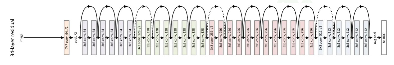
Figure 1. Full architecture of a ResNet model, here with 34 layers. ResNet-50 and 200 slightly differ from this one as the two 3x3 convolutions of each block are replaced by a 1x1, a 3x3 and a 1x1 convolution.
From ResNet to ConvNeXt
Training techniques
Before digging into the changes of the model itself, the idea is to take advantage of modern training techinques, as the training procedure also effects the ultimate performance of the model. They used AdamW optimizer instead of standard SGD, increased the training duraring from 90 to 300 epochs and employed many data augmentation strategies – Mixup, Random Erasing or Label Smoothing to name only few of them. This new training procedure increase the performances of the ResNet-50 from 76.1% of accuracy (baseline, taken from the original ResNet paper) to 78.8%. It is kept as it for the rest of the study.
Macro Design
Stage compute ratio
Both in Swin and ConvNets, the feature map resolution changes at the different stages of the network. For Swin, the compute ratio of the stages is 1:1:3:1, and it increases to 1:1:9:1 for larger Swin models. Following this, they changed the number of blocks in each stage of the ResNet-50 from (3,4,6,3) to (3,3,9,3), resulting in an improvment of the model accuracy to 79.4%.
Changing ‘stem cell’
Stem cell refers to how the input images will be processed by the first convolutions of the network. In the original ResNet, is it done with a 7x7 with stride 2 and a max pooling operation, resulting in a downsampling of a factor 4. In Vision Transformers, it is done using non-overlapping convolutions. When replacing the standard ResNet stem cell by a a simpler convolution of size 4 and stride 4, the accuracy increases from 79.4% to 79.5%.
ResNeXt-ify
A special type of convolutions, called grouped convolutions, gathers convolutional filters into separated groups. It is known to have a better FLOPs/accuracy trade-off and has already been used in several ConvNets like ResNeXt.
Here, the authors use a special type of grouped convolution, called depthwise convolution, where individual convolutions have a depth of 1 and there are as many convolution as channels. When precesseding a 1x1 convolution, it creates a separation of the spatial and channel information mixing, a property that is present in vision Transformers. Using this type of convolutions resulted in a drop of accuracy but also of the FLOPs, allowing to increase the reference number of channels from to 64 to 96. It the end, these changes made the accuracy reaches 80.6%.

Figure 2. Illustration of the combination of depthwise convolution and a 1x1 convolution for a 3-channel image.
Inverted Bottleneck
In Transformer blocks, the MLP block generally has a higher hidden dimension than the input, the standard ratio being 4. This kind of inverted bottleneck was not so common in ConvNets architectures, but recent works have shown its interest and it is used in several advanced convolutional architectures. This design choice slightly improved the accuracy of the modified ResNet from 80.5% to 80.6%.
Large Kernel Sizes
One of the main characteristics of Vision Transformers is their non-local attention computation. Even in more recent versions like Swin, where the attention is not computed between all the patches to limit the complexity, the windows size is at least 7x7. On the other hand, in ConvNets, the kernel size of the convolutions is generally much smaller, as the most common value used is 3x3. Investigations conducted by the authors on kernel sizes showed that, for this model, increasing the kernel size improve the accuracy. However, a too large kernel size may not be beneficial as the peak performance was achieved with 7x7 kernels and using larger kernels (sizes of 9 and 11) did not result in better performances. Hence, the kernel size for depthwise convolutions was set to 7x7.
Micro Design
After having fixed the architecture of the model at a macro and at a block level, the authors focus on some micro design choices concerning activation functions and batch normalization.
Type and number of activation functions
Like if many advanced Transformers used for NLPs and ViT-like models, the authors adopted the GELU activation function, defined by \(\text{GELU}(x) = 0.5x(1+\text{erf}(\frac{x}{\sqrt{2}}))\), even though the performances remained unchanged compared to when using the standard ReLU activation. In ConvNets, the standard practice is to append an activation function to each convolutional layer, while in Transformers, there is only one, in the MLP block. They tried to reduce the number of activation per ResNet block to only one between the two 1x1 convolution and this change increased the performances to 81.3% of accuracy.
Type and number of normalization layers
Transformers blocks also usually have fewer normalization layers than ConvNets. The authors left only one of these layers before the 1x1 convolutional layers and substituted the Batch Normalization layer that was used in ResNet with a Layer Normalization. Again, these modifications boosted the performances of the model to 81.5% of accuracy on ImageNet-1K.
The Fig. 3 summarizes how the micro design choices have modified the the standard ResNet Block to obtain the final version of ConvNeXt’s main block.

Figure 3. Summary of the steps that have been looked over to modernize ResNet.
Downsampling layers
Finally, the authors also changed how the downsampling is performed in ResNet. In the latter, it is included in the first block of each stage as the first 3x3 convolution has a stride of 2. They swapped this for a separate 2x2 convolution with a stride of 2 at the beginning of each stage. At this point, they had to add a few more normalization layers before each downsampling layer because the training was diverging.
This is the last change that was adopted to get the final ConvNeXt model. It reached a score of 82.0%, significantly outperforming Swin-T and its 81.3% of accuracy.
As a summary of the design choices that trajectory followed by the authors, the figure below summarizes the design choices that have been tested and their associated performances and GFLOPs.
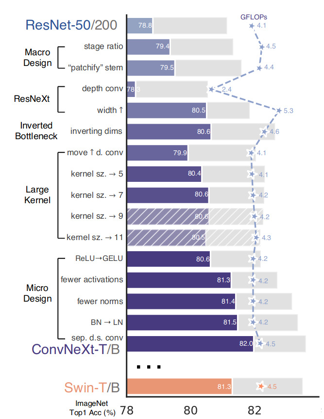
Figure 4. Summary of the steps that have been looked over to modernize ResNet.
Results with ResNet-200 basis and Swin-B are shown with gray bars. A hatched bar means the modification was not adopted.
Evaluation on other tasks and scalability
As mentioned earlier, all the design choices have been tested and approved or not on ResNet-50 and ResNet-200 based on the performances obtained for a classification task on ImageNet-1K. In order to see whether or not the model scales well and how it performs on other tasks, they made other versions of ConvNeXt, matching Swin-S, and Swin-L FLOPs and number of parameters, and uses them as backbone architectures for object detection and semantic segmantion.
They fine-tuned Mask R-CNN and Cascade Mask R-CNN on the COCO dataset and UperNet on the ADE20K semantic segmentation task. The next two figures shows the performances of these models compared to their Swin counterpart. For both tasks and all model sizes, ConvNeXt’s performances are in par or better than Swin’s.
Many more experiences and results are shown in the article, as well as the detail of the architecture of the models.

Figure 5. Performances of ConvNeXt and Swin models when used as backbone with Mask-RCNN and Cascade Mask-RCNN for COCO object detection task. All the models are pre-trained on ImageNet-1K except the last five, that are pre-trained on ImageNet-22K.

Figure 6. Performances of ConvNeXt and Swin models when used as backbone with UperNet for ADE20K semantic segmentation task
Conclusion
The authors have proposed a pure convolutional neural network called ConvNeXt that aim to be a generic backbone for computer vision tasks. They achieved state-of-the-art performances on several classic tasks, surpassing Hierarchical Transformers such as Swin. The most impressive part of their proposal is that they did not introduce any new concept or design, but only examined many design choices that have been proposed and studied seperately over the past decade on ConvNets and Transformers and merged them to get this new architecture.