ConvNeXt V2: Co-designing and Scaling ConvNets with Masked Autoencoders
Notes
- Important : See this review to understand ConvNeXt V1
- Also you can refer to this review about Masked Autoencoders (MAE)
Highlights
- ConvNeXt V1 was focused on supervised learning only. However, similarly to transformers, convolution based models can benefit from self-supervised learning techniques (such as MAE)
- Simply applying self-supervised learning methods (i.e. MAE) to ConvNeXt leads to sub optimal results
- This article proposes a fully convolutional masked autoencoder framework (MAE) and modifies the ConvNeXt architecture with Global Response Normalization (GRN) layers
Fully convolutional masked autoencoder
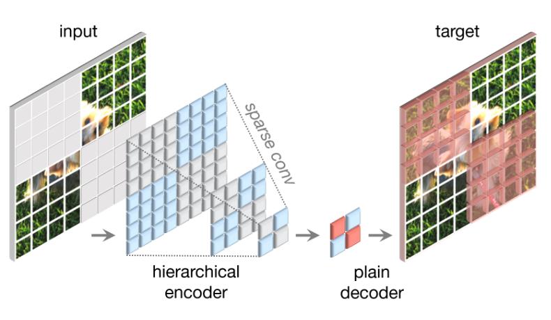
Figure 1 : Fully convolutional masked autoencoder design
-
They use a random masking strategy with a masking ratio of 0.6
-
They use ConvNeXt as the encoder
-
Unlike transformers you can’t simply remove masked patches from the image as the 2D structure of the image must be preserved for convolution
-
Also naive solutions such as replacing masked patches by masked tokens don’t perform well in practice
-
The idea here is to see the masked image as sparse data. Based on that, it is natural to use sparse convolution that will operate only on visible pixels
Note 1 : if the center pixel of the convolution is masked then the convolution will not operate and just return a masked pixel
Note 2 : sparse convolution layers can be converted back to standard convolutions at the fine-tuning stage without requiring additional handling
-
They tested several decoder architectures/depths but at the end they chose a simple ConvNeXt plain decoder
-
Loss function is the mean squared error (MSE) computed only on the masked patches between reconstructed and target images
Evaluation of FCMAE
-
They pre-train and fine-tune on ImageNet-1K for 800 and 100 epochs respectively and report top-1 accuracy
-
Ablation study is done to justify design choice

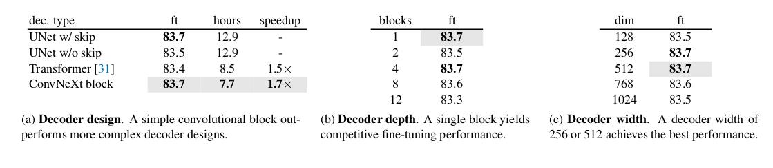
Figure 2 : Results of the FCMAE’s ablation study
-
The also compare the self-supervised approach to fully supervised learning
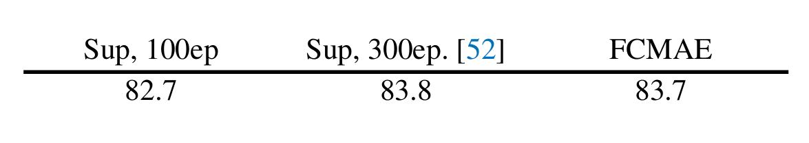
Figure 3 : Comparison with fully supervised approach
-
They perform better than the fully supervised setup trained for 100 epochs but are still worse than the orginal ConvNeXt V1 baseline trained for 300 epochs
This is in contrast to the recent success of masked image modeling using transformer-based models [..] where the pre-trained models significantly outperform the supervised counterparts.
Global Response Normalization
- To try to improve on that and to gain more insight into the learning behavior they perform a qualitative analysis in the feature space.

Figure 4 : illustration of the feature collapse phenomenom
-
They noticed a feature collapse phenomenon and they computed the cosine distance between features to get more insight
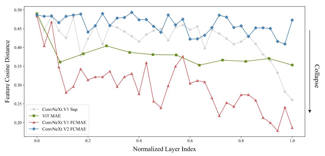
Figure 5 : Cosine distance between features for all models
Note : ConvNeXt V2 FCMAE is the new architecture which is the ConvNeXt V1 FCMAE with the new normalization layer added to fix the feature collapse phenomenon
-
This analysis showed a reduction in feature diversity through the network for the ConvNeXt V1 FCMAE model
-
They propose to introduce a new normalization layer called global response normalization (GRN) to increase feature diversity
-
This layer is composed of three steps:
-
global feature aggregation : consists of mapping each feature map \(X_i\) into a scalar and constructing a vector representing all feature maps
Here they use the \(L2\)-norm : \(G(X) = \lbrace \Vert X_1 \Vert, \Vert X_2 \Vert, ...,\Vert X_C \Vert \rbrace\)
-
feature normalization : \(N( \Vert X_i \Vert) = \frac {\Vert X_i \Vert}{\sum_{j=1,...,C} \Vert X_j \Vert}\)
-
feature calibration : \(X_i = X_i * N(G(X)_i)\)
-
-
They add a residual connection to create the final block which is: \(X_i = \gamma * X_i * N(G(X)_i) + \beta + X_i\), with \(\gamma\) and \(\beta\) learnable parameters
-
They incorporate the GRN layer into the ConvNeXt block creating ConvNeXt V2
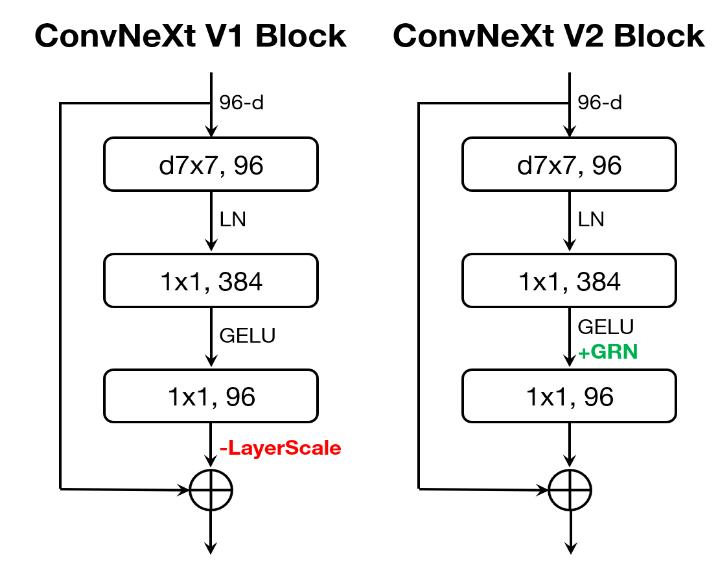
Figure 6 : Illustration of ConvNeXt block
Impact of GRN
- GRN succeeds to mitigate the feature collapse behavior (see cosine distance between features maps)
- The new model outperforms the 300 epochs supervised counterpart

Figure 7 : Result of ConvNeXt V2
-
Ablation study
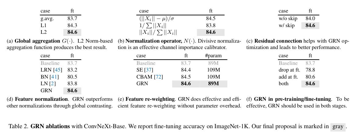
Figure 8 : Ablation study of GRN layer
ImageNet Experiments
Classification
- Comparison with ConvNeXt V1 and contribution of pre-training:
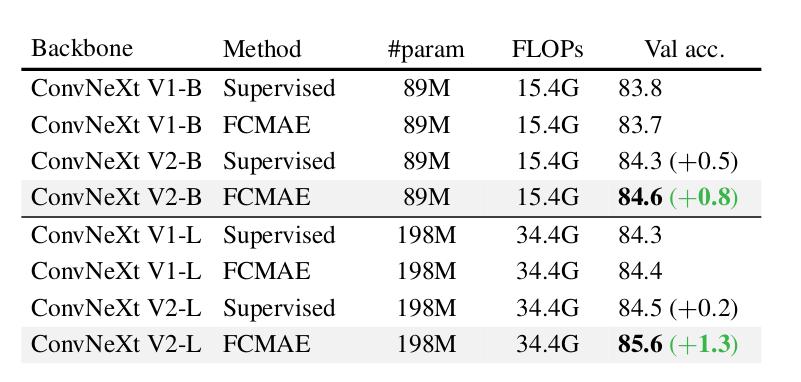
Figure 9 : Detailed results

Figure 10 : Comparison with SOTA methods
- They also evaluate the performance of the framework when adding an intermediate pretraining on Image-net 22K
- They achieve the best state of the art results on Image-Net 1K using only public dataset
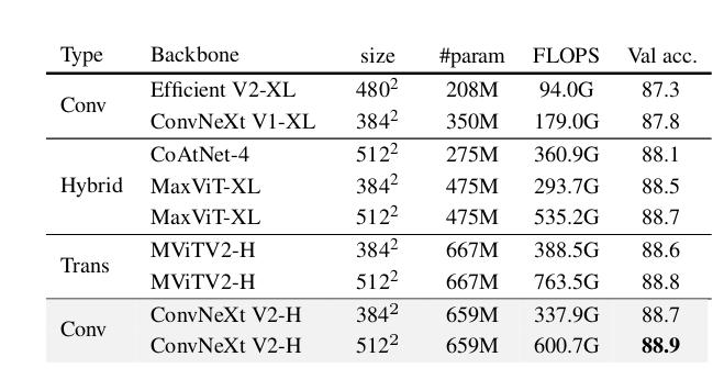
Figure 11 : Results with intermediate pretraining on Image-Net 22K
Object Detection

Figure 12 : Object detection results
Semantic Segmentation

Figure 13 : Semantic segmentation results
Conclusion
The fully convolutional masked autoencoder pre-training allows to improve the performance on various tasks but requires a specific architecture design.