Variational Dropout and the Local Reparameterization Trick
Notes
- Link of a useful video: video
- This post was made to establish the basis of variational dropout for a future post on sparse variational dropout.
Highlights
- The objective of this paper is to have Bayesian posterior over the neural network parameters.
- It is also introducing the Local Reparameterization trick
- Finally, both previous points help to developp variational dropout
Introduction
As is well known nowadays, deep neural networks can scale to millions of parameters. However, this flexbility may lead to overfitting, and therefore decrease robustness on new data. Various regularization techniques are used in practice, such as dropout.
In a previous paper that they cite, it was shown that binary dropout has a Gaussian approximation called Gaussian dropout. Based on that, they show that a relationship exists between dropout and Bayesian inference to greatly improve the efficiency of variational Bayesian inference on the model parameters. The problem they underline is that :
Bayesian methods for inferring a posterior distribution over neural network weights have not yet been shown to outperform simpler methods such as dropout.
That’s why they proposed a new trick called the Local reparameterization trick that will improve the stochastic gradient based variational inference with minibatches of data thanks to the translation of global uncertainty into a local noise. Their method leads to an optimization speed on the same level as fast dropout and allows a full Bayesian analysis of the model.
Method
Bayesian inference on model parameters
Let’s have a dataset \(\mathcal{D}\) containing \(N\) observations of tuples \((\textbf{x},\textbf{y})\).
The goal in the paper is to learn a model with weights \(\textbf{w}\) of the conditional probability \(p(\textbf{y} \vert \textbf{x}, \textbf{w})\). This is a generic example, the method they propose can be applied to standard classification or regression or other types of models (like unsupervised models).
Basically, they try to learn \(p(\textbf{w} \vert \mathcal{D}) = p(\textbf{w}) p(\mathcal{D} \vert \textbf{w}) / p(\mathcal{D})\). However, this true posterior is intractable that’s why they will try to have the best approximation by minimizing :
\[D_{KL}(q_{\phi} (\textbf{w}) \vert \vert p(\textbf{w} \vert \mathcal{D}))\]/!\ with \(q_{\phi} (\textbf{w})\) (confusing notation) :
- \(\phi\) represents the parameters of the distribution (for exemple \(\mu\) and \(\sigma\))
- \(\textbf{w}\) represents the parameters or weights of the model
Finally they have :
\[\mathcal{L}(\phi) = - D_{KL}(q_{\phi} (\textbf{w}) \vert \vert p(\textbf{w})) + L_{\mathcal{D}}(\phi)\] \[L_{\mathcal{D}}(\phi) = \sum_{(\textbf{x},\textbf{y}) \in \mathcal{D}} \mathbb{E}_{q_{\phi} (\textbf{w})} log(p(\textbf{y} \vert \textbf{x},\textbf{w}))\]
Local Reparameterization Trick
What they explain in section 2.1 and 2.2 in the paper is that they can estimate the gradient of the log-likelyhood with Monte-Carlo based method. It is also possible to do it to approximate the KL divergence. But in practice the performance of stochastic gradient ascent crucially depends on the variance of the gradients. They show that the variance of \(L_{\mathcal{D}}^{SGVB}(\phi)\) (where SGVB stands for Stochastic Gradient Variational Bayes, defined in their previous paper here) can be dominated by the covariances for even moderately large \(M\) (size of the minibatch).
\[Var \left[ L_{\mathcal{D}}^{SGVB}(\phi) \right] = N^2 \left( \frac{1}{M} Var \left[ L_i \right] + \frac{M-1}{M} Cov \left[ L_i, L_j \right] \right)\]\(L_i = log( p(\textbf{y}^i \vert \textbf{x}^i, \textbf{w} = f (\epsilon^i, \phi)))\) (contribution to the likelihood for the \(i\)-th datapoint in the minibatch)
Therefore they introduce the Local Reparameterization Trick to solve this issue.
To do so they propose a new estimator where the aim is to have \(Cov \left[ L_i, L_j \right] = 0\) so that the variance of the stochastic gradients scales as \(1/M\).
Exemple taken in the paper :
Consider a standard fully connected neural network containing a hidden layer consisting of 1000 neurons. This layer receives an \(M\) x \(1000\) input feature matrix \(\textbf{A}\) from the layer below, which is multiplied by a \(1000\) x \(1000\) weight matrix \(\textbf{W}\), before a nonlinearity is applied, i.e. \(\textbf{B = AW}\). We then specify the posterior approximation on the weights to be a fully factorized Gaussian, i.e. \(q_\phi(w_{i,j}) =N (\mu_{i,j}, \sigma_{i,j}^2) \forall w_{i,j} \in \textbf{W}\), which means the weights are sampled as \(w_{i,j} = \mu_{i,j} + \sigma_{i,j} \epsilon_{i,j}\), with \(\epsilon_{i,j} \sim \mathcal{N}(0, 1)\). In this case we could make sure that \(Cov [L_i,L_j]=0\) by sampling a separate weight matrix \(\textbf{W}\).
This approach is not computationally efficient. To make it so they applied another trick:
\[q_\phi(w_{i,j}) =N (\mu_{i,j}, \sigma_{i,j}^2) \forall w_{i,j} \in \textbf{W} \Rightarrow q_\phi(b_{m,j}) =N (\gamma_{m,j}, \delta_{m,j})\]Fortunately, the weights (and therefore \(\epsilon\)) only influence the expected log likelihood through the neuron activations \(\textbf{B}\), which are of much lower dimension. If we can therefore sample the random activations \(\textbf{B}\) directly, without sampling \(\textbf{W}\) or \(\epsilon\), we may obtain an efficient Monte Carlo estimator at a much lower cost. For a factorized Gaussian posterior on the weights, the posterior for the activations (conditional on the input \(\textbf{A}\)) is also factorized Gaussian
with
\(\gamma_{m,j} = \sum_{i=1}^{1000} a_{m,i}\mu_{i,j}\) and \(\delta_{m,j} = \sum_{i=1}^{1000} a_{m,i}^2\sigma_{i,j}^2\)
Rather than sampling the Gaussian weights and then computing the resulting activations, we may thus sample the activations from their implied Gaussian distribution directly, using \(b_{m,j} = \gamma_{m,j} + \sqrt{\delta_{m,j}}\zeta_{m,j}\), with \(\zeta_{m,j} \sim \mathcal{N}(0, 1)\).
Here, \(\zeta\) is an \(M \times 1000\) matrix, so only \(M \times 1000\) random variables have to be sampled instead of \(M \times 1\,000\,000\).
The local reparameterization trick leads to an estimator that has lower variance and is more computationally efficient.
Variational Dropout
Dropout consists of adding multiplicative noise to the input of each layer. For a fully connected layer we have :
\(\textbf{B} = (\textbf{A} \circ \xi)\theta\) with \(\xi \sim p(\xi_{i,j})\)
- \(\textbf{A}\) is the \(M\) x \(K\) matrix of input features
- \(\theta\) is a \(K\) x \(L\) weight matrix
- \(\textbf{B}\) is the \(M\) x \(L\) output matrix
It was shown in a previous paper that using a continuous distribution such as a Gaussian \(\mathcal{N}(1,\alpha)\) with \(\alpha = \frac{p}{(1-p)}\) works as well or batter than a Bernoulli distribution with a probability \(1-p\) (with \(p\) the dropout rate).
Variational dropout with independent weight noise
If the elements of the noise matrix \(\xi\) are drawn independently from a Gaussian \(N (1, \alpha)\), the marginal distributions of the activations \(b_{m,j} \in \textbf{B}\) are Gaussian as well:
\(q_\phi(b_{m,j} \vert \textbf{A}) = N (\gamma_{m,j}, \delta_{m,j})\) with \(\gamma_{m,j} = \sum_{i=1}^{K} a_{m,i}\theta_{i,j}\) and \(\delta_{m,j} = \alpha \sum_{i=1}^{K} a_{m,i}^2\theta_{i,j}^2\)
With this equation, the activations are directly drawn from their (approximate or exact) marginal distributions.
This Gaussian dropout noise can be seen as a Bayesian treatment of a neural network with \(\textbf{B = AW}\) where the posterior distribution of the weights is given by a factorized Gaussian with :
\[q_\phi(w_{i,j}) = \mathcal{N}(\theta_{i,j}, \alpha\theta_{i,j}^2)\]The paper includes another section on variational dropout with correlated weight noise, but we do not developp it in this post.
Dropout’s scale-invariant prior and variational objective
The aim of this section in the paper is to find an approximation of the variational objective function. They show that the posterior \(q_\phi(\textbf{W})\) can be decomposed into 2 parameters :
- \(\theta\) for the mean
- the multiplicative noise determined by \(\alpha\)
During dropout training, \(\theta\) is adapted to maximize the expected log likelihood \(\mathbb{E}_{q_{\alpha}} \left[ L_{\mathcal{D}}(\theta) \right]\). For this to be consistent with the optimization of a variational lower bound, the prior on the weights \(p(\textbf{w})\) has to be such that \(D_{KL}(q_\phi(\textbf{w}) \vert \vert p(\textbf{w}))\) does not depend on \(\theta\).
They show that the only prior possible is :
\[p(log(\vert w_{i,j} \vert)) \propto c\]Therefore, they try to maximize :
\[\mathbb{E}_{q_{\alpha}} \left[ L_{\mathcal{D}}(\theta) \right] - D_{KL}(q_\alpha(\textbf{w}) \vert \vert p(\textbf{w}))\]- \(\theta\) and \(\alpha\) are treated as hyperparameters that are fixed during training.
However, \(- D_{KL}(q_\alpha(\textbf{w}) \vert \vert p(\textbf{w}))\) is analytically intractable but can be approximated by :
\[- D_{KL} \left[ q_\phi(w_i) \vert \vert p(w_i) \right] \approx constant + 0.5log(\alpha) + c_1\alpha + c_2\alpha^2 + c_3\alpha^3\]with
\[c_1 = 1.16145124, c_2 = -1.50204118 , c_3 = 0.58629921\]Now that there is a derived dropout’s variational objective, they show that maximizing the variational lower bound with respect to \(\alpha\) will make the hyperparameters \(\alpha\) and \(\theta\) adaptative. Furthermore, it will be possible to learn a separate dropout rate per layer, per neuron, or even per separate weight.
Despite this new approach, they have found that large values of \(\alpha\) will imply large-variance gradients. That’s why they apply a constraint on \(\alpha\) (\(\alpha \le 1\) i.e.* \(p \le 0.5\)) during training.
We will show in future post on sparse variational dropout that this constraint can be removed, leading to sparse representation of neural networks.
Results
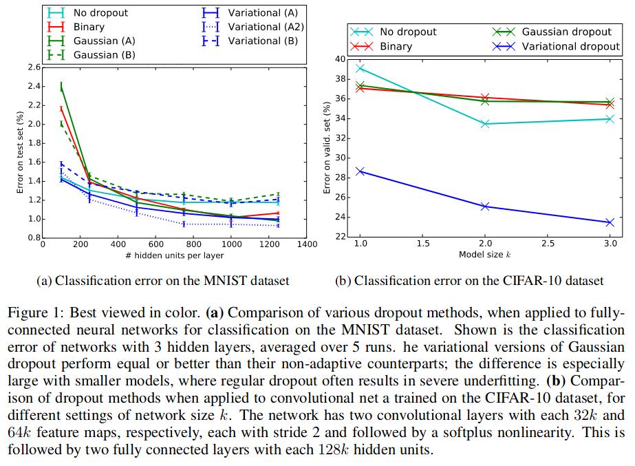
Comparison of their method to standard binary dropout and two versions of Gaussian dropout.
- Gaussian dropout A : pre-linear Gaussian dropout1
- Gaussian dropout B : post-linear Gaussian dropout2
Two types of variational dropout as well :
- Variational dropout A : correlated weight noise (equivalent of an adaptative Gaussian dropout type A)
- Variational dropout A2 denotes performance of type A variational dropout but with a KL-divergence downscaled with a factor of 3 (seems to prevent underfitting)
- Variational dropout B : independant weight noise (equivalent of Gaussian dropout B)
Tests were done on MNIST dataset for a classification task. They used the same architecture and drop rate as in the original dropout paper1, with the drop rate corresponding to \(p \le 0.5\) for the hidden layers and \(p \le 0.2\) for the input layer.
Conclusion
-
They obtained an efficient estimator with a low computational complexity and a low variance by injecting noise locally instead of globally.
-
They show that dropout is a special case of SGVB with local reparameterization leading to variational dropout, where optimal dropout rates are inferred from the data, rather than fixed in advance.
References