Regularized Evolution for Image Classifier Architecture Search
What is Neural Architecture Search?
Neural Architecture Search (NAS) [1] is a machine learning field dealing with the automation of neural network architecture design. Its main motivation is to avoid the time-consuming step of manually designing neural network architectures.
NAS requires three main elements to output a high-performing neural network for a specific task:
- The Search Space defines the set of architectures that are considered. Usual search spaces include:
- Macro search spaces (high representation power, slow to search)
- Chain-structured search-spaces (low representation power, quick to search)
- Cell-based search spaces
- Hierarchical search spaces
- (…)
- The Search Strategy defines the method to find well-performing architectures in the search space.
- Reinforcement Learning
- Evolutionary methods
- Bayesian Optimization
- One-shot methods (more efficient but less robust)
- (…)
- The Performance Estimation Strategy defines the method used to evaluate a given architecture. The goal here is to avoid running a full training of each architecture to save time and computational resources.
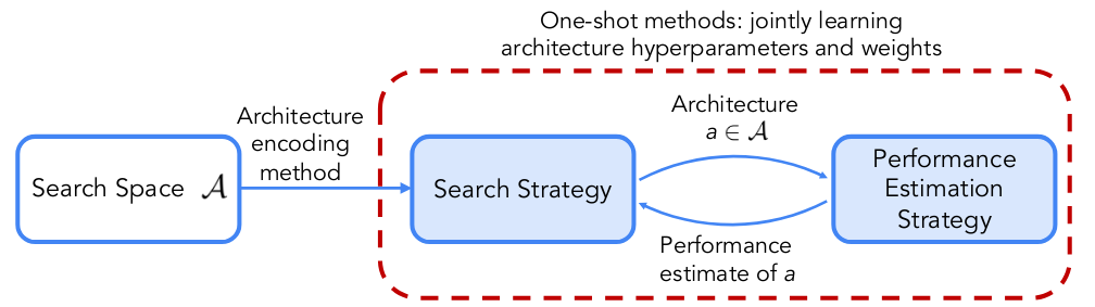
Figure 1: Building blocks of NAS
NAS can then be defined as:
Given a search space A, a dataset D, a training pipeline P, and a time or computation budget t, the goal is to find an architecture a ∈ A within budget t which has the highest possible validation accuracy when trained using dataset D and training pipeline P.
In this paper, the authors develop AmoebaNet-A, the first evolved NAS network to achieve state-of-the-art performance on ImageNet in 2019.
Application to Image Classification
The goal of the paper is to develop an evolved NAS model that:
- achieves state-of-the-art performance (as of 2019) on ImageNet.
- is faster than the best RL-based NAS model (NASNet [2]).
Search Space
They use the NASNet search space [2], a cell-based search space of image classifiers that consists in a feed-forward stack of inception modules/cells.
Each cell receives an input of the previous cell and a skip input from the cell that came before that. There are two type of cells: normal and reduction cells. The latter are followed by a stride of 2 to reduce the image size. All normal (resp. reduction) cells have the same architecture. Each cell receives two inputs and computes one output through five pairwise combinations.
Each pairwise combination takes two inputs and computes one output. It consists of applying an operation to each input and adding the results. Once five combinations are selected, the unused hidden states are concatenated to form the cell output. Possible operations are:
- 3x3, 5x5, 7x7 separable convolution
- 3x3 average pooling
- 3x3 max pooling
- 3x3 dilated separable convolution
- 1x7 then 7x1 convolution
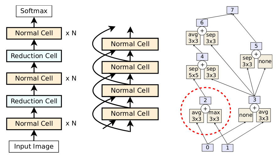
Figure 2: NasNET search space. LEFT: the full outer structure (omitting skip inputs for clarity). MIDDLE: detailed view with the skip inputs. RIGHT: cell example. Dotted line demarcates a pairwise combination.
For this search space, the goal is to find the best architecture of normal and reduction cells and there are two parameters to set manually to define the size of the network: the number of stacked normal cells (N) and the number of filters of the convolution operations in the first stack (F).
Evolutionary Algorithm
They define an evolutionary-based method they call aging evolution in which they “keep a population of N models and proceed in cycles: at each cycle, copy-mutate the best of S random models and kill the oldest in the population”.
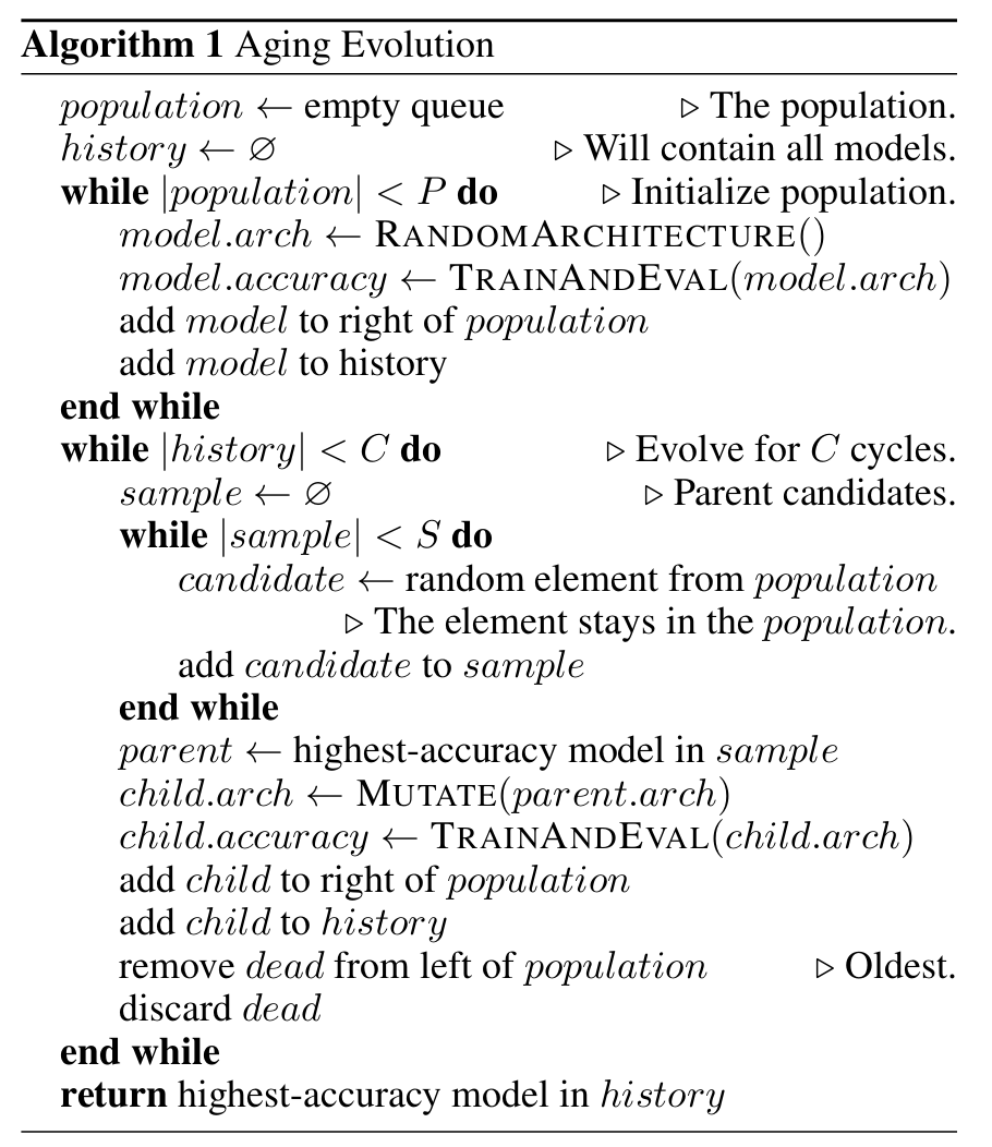
Pseudocode describing the evolutionary-based method.
They consider two mutation types:
- Hidden state mutation: pick either normal or reduction cell, pick one of the five pairwise operations, pick one of the elements of the pair, replace its hidden state with another one within the cell.
- Op mutation: pick either normal or reduction cell, pick one of the five pairwise operations, pick one of the elements of the pair, replace the operation with a random one.
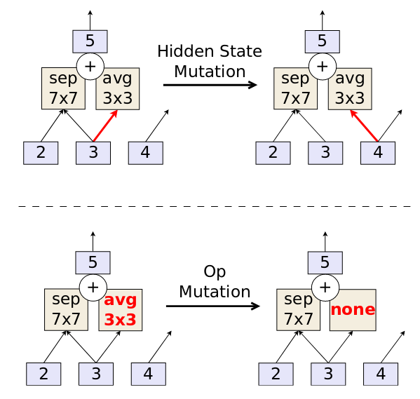
Figure 3: Illustration of the two mutation types.
There are three parameters to set manually: the population size P, the sample size S and the total number of models C. There are as well the hyperparameters for the training of each network.
Experimental Setup
The evolutionary architecture search is performed on the CIFAR-10 dataset over small N and F values (N=3 and F=24) and networks are trained over 25 epochs before evaluating them. They use P=100 and S=25. The procedure is stopped when 20,000 models are evaluated. Then, the best evolved architecture is selected and N and F are increased (N=6 and F=190/448) to obtain an enlarged architecture that is then trained on CIFAR-10 or transferred to ImageNet for a standard training with 600 epochs.
Results

Figure 4: AmoebaNet-A architecture. The overall model (LEFT) and the AmoebaNet-A normal cell (MIDDLE) and reduction cell (RIGHT).

Figure 5: Time-course of 5 identical large-scale experiments for each algorithm (evolution, RL, and RS), showing accuracy before augmentation on CIFAR-10. All experiments were stopped when 20k models were evaluated, as done in the baseline study.

Figure 6: Final augmented models from 5 identical architecture-search experiments for each algorithm, on CIFAR-10. Each marker corresponds to the top models from one experiment.

Table 1: ImageNet classification results for AmoebaNet-A compared to hand-designs (top rows) and other automated methods (middle rows). The evolved AmoebaNet-A architecture (bottom rows) reaches the current state of the art (SOTA) at similar model sizes and sets a new SOTA at a larger size. All evolution-based approaches are marked with a ∗.
Discussion
- Model speed.
- Asynchronous evolution is used to optimize resource utilization (i.e., parallelization of evolution). This favors the reproduction of fast models.
- Aging evolution.
- Comparing aging and non-aging evolution, the former seems better. This may be explained by thinking of aging evolution as a form of regularization of the search space. In non-aging evolution, models that that obtain good results by luck may stay in the population for a long time and introduce noise by producing many children. By progressively killing old models, this type of noise is avoided.
- Interpreting architecture search.
- NAS can help discover new neural network design patterns.
Conclusions
- AmoebaNet-A achieved state-of-the-art results on ImageNet.
- Enlarged AmoebaNet-A set a new state-of-the-art on ImageNet.
- Compared to RL, evolution performs faster architecture search.