Learning Loss for Active Learning
Highlights
- This paper proposes a simple active learning method with a loss prediction module added to the target module.
- It is not task-specific and can be applied to any sort of task.
- The method is tested on three computer vision tasks that are image classification, object detection and human pose estimation.
Introduction
Despite progress, deep networks still require more and more data, and their performance is still not saturated with respect to the size of the training data. But labelling data is expensive -even more so in medical imaging, where experts are needed-. Active learning is considered to optimize training in the context of a limited budget for annotation. It consists in selecting specific samples from an unlabelled dataset that are more likely to improve the model than a random sample selection. Selection is usually based on uncertainty, diversity, or expected model change. However, these methods are often task-specific and not always applicable to complex deep learning algorithms.
Proposed solution: a loss prediction module that predicts the loss of unlabelled samples to select those that may not be well predicted.

Definition of the problem
Problematization
The target module \(\hat{y} = \theta_{target}(x)\) is linked to the loss prediction module \(\hat{l} = \theta_{loss}(h)\) where \(h\) is a feature set of \(x\) extracted from several hidden layers of \(\theta_{target}\).
At the begining there is a large pool of unlabelled data \(U_N\) from which \(K\) data points are randomly sampled and annotated to build the initial dataset \(L^{0}_K\) and the unlabelled dataset \(U^{0}_{N-K}\).
The modules \(\theta^0_{target}\) and \(\theta^0_{loss}\) are learned and the whole \(U^{0}_{N-K}\) is evaluated by the loss prediction module in order to get {\((x, \hat{l}) | x \in U^{0}_{N-K}\)}. Then the \(K\) samples with the highest loss are labelled leading to \(L^1_{2K}\) to learn {\(\theta^1_{target} , \theta^1_{loss}\)}.
This process is repeated until performance is satisfactory or the data annotation budget is exhausted.
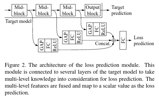
Architecture of the loss prediction module
The goal is to build a loss prediction module that is independant to the considered task as it imitates the target model loss. Moreover, it must be small as the computational cost of the target module is often already high. Both modules are trained jointly so it does not require supplementary training.
The loss prediction module takes multi-layer features maps \(h\) extracted from mid-blocks of the target module as input. Each of them are reduced to a fixed dimensional feature vector through a global average pooling layer and a fully-connected layer before being all concatenated and pass through another fully-connected layer. The output is a scalar value \(\hat{l}\) as predicted loss.
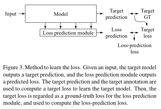
Loss of the loss prediction module
The goal is to learn {\(\theta^s_{target}, \theta^s_{loss}\)} from \(L^s_{(s+1)K}\) defined as \(\hat{y} = \theta_{target}(x)\) and \(\hat{l} = \theta_{loss}(h)\).
The loss of the target task can be defined as \(l = L_{target}(\hat{y},y)\) which is the ground truth for the loss module prediction for the sample \(h\) so we have \(l'=L_{loss}(\hat{l},l)\). The final loss function to learn both modules is
\[L_{target}(\hat{y},y) + \lambda L_{loss}(\hat{l},l)\]where \(\lambda\) is a scaling constant.
A way to define the loss prediction loss function is the MSE: \(L_{loss}(\hat{l},l) = (\hat{l}-l)^2\) but it is not suitable as the scale of the real loss changes through the learning process. The loss function must discard the overall scale of \(l\). The proposed solution is to compare pairs of samples.
Considering the mini-batch \(B^s \in L^s_{(s+1)K}\) of size B, B/2 pairs of data are made such as {\(x^p = (x_i,x_j)\)}. The loss prediction module is learned considering the difference between a pair of loss predictions.
\[L_{loss}(\hat{l_p}, l_p) = max(0, -𝟙(l_i,l_j) (\hat{l_i}-\hat{l_j}) + \xi) \quad where \quad 𝟙(l_i,l_j) = \left\{ \begin{array} +1 \quad if \quad l_i>l_j \\ -1 \quad otherwise \end{array} \right.\]and \(\xi > 0\) is predefined. If \(l_i>l_j\) the loss is zero unless \(\hat{l_j} + \xi > \hat{l_i}\) forcing \(\hat{l_i}\) to increase and \(\hat{l_j}\) to decrease.
All together for the mini-batch \(B^s\) in active learning stage \(s\), the total loss is
\[\frac{1}{B} \sum_{(x,y) \in B^s} L_{target}(\hat{y},y) + \lambda \frac{2}{B} \sum_{(x,y) \in B^s} L_{loss}(\hat{l^p},l^p)\]where \(\hat{y} = \theta^s_{target}(x) \quad \hat{l^p} = \theta^s_{loss}(h^p) \quad and \quad l^p = L_{target}(\hat{y^p},y^p)\)
The loss prediction module will pick up the most informative data points and asks human oracle to annotate them for the next active learning stage \(s+1\).
Application to computer vision tasks
| Task | Image classification | Object detection | Human pose estimation |
|---|---|---|---|
| Dataset | CIFAR-10 50000 images train, 10000 images test |
PASCAL VOC 2007 & 2012 16551 images train, 4952 images test |
MPII 14679 images train, 2729 images test |
| Architecture | ResNet 18 | Single Shot Multibox detector with VGG 16 backbone | Stacked Hourglass Network |
| Training particularities |
At each cycle a subset \(S_M \in U_N\) is considered among which the \(K\) more incertain are taken \(M=10000\) Classic data augmentation |
At each cycle a subset of the unlabeled data is taken \(S_M \in U_N\) \(M=5000\) | |
| Hyper- parameters |
200 epochs Mini-batch size 128 Learning rate 0.1 for the 160 first epochs then 0.01 \(\lambda = 1\) |
300 epochs Mini-batch size 32 Learning rate 0.001 for the first 240 epochs then 0.0001 \(\lambda = 1\) |
125 epochs Mini-batch size 6 Learning-rate 0.00025 for the first 100 epochs then 0.000025 \(\lambda = 0.0001\) |
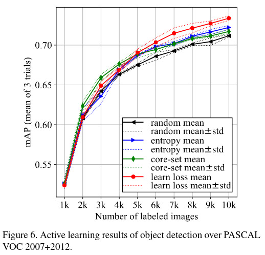
| Evaluation metric | Classification accuracy | mean Average Precision | PCKh@0.5 |
| Results | 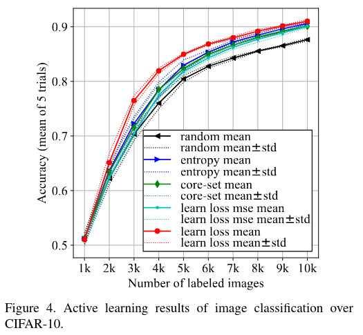 |
 |
 |
Discussion
A new active learning method is introduced applicable to several tasks and deep learning. However diversity and density of data is not considered, taking them into account could help increase the accuracy of loss prediction that was still low in complex tasks.