Deep Unfolded Robust PCA with Application to Clutter Suppression in Ultrasound
Context
Contrast-enhanced ultrasound imaging (CEUS) allows to visualise blood vessels to assess several clinical conditions. It makes use of gas microbubbles as an ultrasound contrast agent that is injected in the vascular system.
What is clutter?
- The slow movement of tissue generates high-amplitude, low-frequency signal, called clutter, that corrupts the underlying blood signal. A filter needs to be applied to remove clutter signal without destroying blood information.

Spectral scheme of blood and tissue signal.
- Traditionally, clutter was removed with high-pass filters, making use of the temporal information of the signal.
- In order to make use of spatial information as well, a filter based on the Singular Value Decomposition (SVD) of the signal was introduced, making use of the high spatial coherence of tissue signal and the low spatial coherence of blood signal. However, this method requires to set a parameter manually.
Problem formulation
An ultrasound signal D is acquired. where \(D \in \mathbb{C}^{M \times M \times T}\) can be decomposed in three signals:
\[D = L + S + N,\]where L is the tissue signal, S is the blood signal and N is the noise signal. All matrices can be rewritten to have shape \(M^2 \times T.\) In the context of contrast-enhanced ultrasound imaging, and if the matrices are reshaped as \(M^2 \times T\) such that the columns carry the temporal information, some assumptions can be made about L and S:
- L is low-rank because of the spatial coherence of tissue signal
- S is sparse because of the low proportion of blood vessels in the image
The decomposition of a matrix in low-rank and sparse components is called Robust Principal Component Analysis (RPCA) [1] and L and S can be found solving a convex minimization problem.
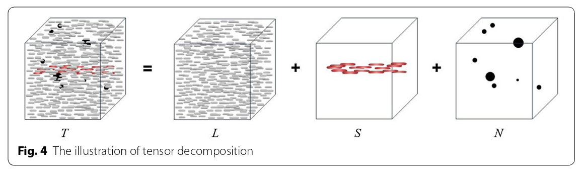
Figure from [2].
How to solve this problem?
The authors provide three ways to find matrix S.
- Model-based method, solved with an:
- Iterative algorithm.
- Unfolded algorithm.
- Supervised learning:
- ResNet.
Model-based method
The RPCA model written above can be generalized as:
\[D = H_1L + H_2S + N,\]where \(H_1\) and \(H_2\) are measurement matrices. Then, to recover L and S the authors propose the following minimization problem that promotes low-rank solutions for L and sparse solutions for S:
\[\min_{L,S} ||D-(H_1L+H_2S)||^2_F + \lambda_1 ||L||_* + \lambda_2||S||_{1,2},\]where
- \(||\cdot||_F\) is the Frobenius norm (square root of the sum of all squared elements)
- \(||\cdot||_*\) is the nuclear norm (sum of the singular values)
- \(||\cdot||_{1,2}\) is the \(l_{1,2}\) norm (sum of the L2 norms of each row)
Iterative algorithm
This minimization problem can be solved using the Iterative Shrinkage/Thresholding Algorithm (ISTA) [3]. The iterative steps of ISTA are given by:
\[L^{k+1}=\text{SVT}_{\lambda_1/L_f}( (I-\frac{1}{L_f} H_1^T H_1)L^k - H_1^T H_2 S^k + H_1^T D )\] \[S^{k+1}=\mathcal{T}_{\lambda_2/L_f}( (I-\frac{1}{L_f} H_2^T H_2)S^k - H_2^T H_1 L^k + H_2^T D ),\]where
\[\text{SVT}_\alpha(X) = U\text{diag}(\max(0,\sigma_i-\alpha))V^T, \hspace{1cm} i=1, ..., r\]is the singular value thresholding operator where \(X=U\Sigma V^T\) and \(\Sigma=\text{diag}(\sigma_i, ...,\sigma_r),\) and
\[\mathcal{T}_\alpha(x) = \max(0,1-\frac{\alpha}{||x||_2})x\]is the mixed \(l_{1,2}\) soft thresholding operator.

Pseudocode describing the ISTA steps.
The main drawback of this algorithm is that the number of iterations can become high, greatly increasing the algorithm complexity. Also, parameters \(\lambda_1\) and \(\lambda_2\) must be manually set, and \(H_1,\) \(H_2\) and \(L_f\) (the Lipschitz constant of the quadratic term) must be known.
For the experiments, they empirically chose \(\lambda_1=0.02,\) \(\lambda_2=0.001\) and a maximum number of 30,000 iterations.
Unfolded algorithm
The iterative algorithm can be unfolded by replacing matrices dependent on \(H_1\) and \(H_2\) with convolution kernels \(P_1^k,...\) \(P_6^k\) that are learned during training. A neural network can be defined where the operations made at each layer correspond to one ISTA iteration:
\[L^{k+1}=\text{SVT}_{\lambda_1^k}( P_5^k \ast L^k + P_3^k \ast S^k + P_1^k \ast D )\] \[S^{k+1}=\mathcal{T}_{\lambda_2^k}( P_6^k \ast L^k + P_4^k \ast S^k + P_2^k \ast D ).\]The thresholding coefficients are defined at each layer as:
\[\lambda_1^k = \sigma(\lambda_L^k) a_L \max{L^k}\] \[\lambda_2^k = \sigma(\lambda_S^k) a_S \max{S^k},\]where \(\sigma(x)\) is the sigmoid function, \(\lambda_L^k\) and \(\lambda_S^k\) are learned, and they fix \(a_L=0.4\) and \(a_S=1.8.\)
The loss function is the MSE (mean squared error):
\[\mathcal{L}(\theta) = \frac{1}{2n} \sum_{i=1}^n{||f_S(D_i,\theta)-\hat{S}_i||_F^2} + \frac{1}{2n} \sum_{i=1}^n{||f_L(D_i,\theta)-\hat{L}_i||_F^2}.\]The unfolded deep neural network has a total of 1,796 parameters.
Supervised method
As a comparison, they implemented a ResNet consisting of:
- 10 layers.
- First 3 layers used convolution filters of size 5 × 5 × 1 with stride (1, 1, 1), padding (2, 2, 0) and bias, while the last 7 layers used filters of size 3 × 3 × 1 with stride (1, 1, 1), padding (1, 1, 0) and bias.
- ADAM optimizer with a learning rate of 0.002.
- Complex-valued convolutions.
- Total of 25,378 parameters.
Data
The training data consists in:
- both simulated and in vivo (rat brain) data,
- \(32 \times 32 \times 20\) patches that are reshaped into \(1024 \times 20\) patches,
- 4,800 training pairs.
Results
- Results on simulated data: ground-truth vs unfolded.

Simulated data results. (a) MIP (maximum intensity projection) of the input movie (50 frames). (b) Ground-truth blood MIP image. (c) unfolded blood result. (d) Ground-truth tissue MIP image. (e) unfolded tissue result.
- Comparison of the iterative and unfolded methods performance.

MSE as a function of the number of iterations/layers.
- Results on in vivo data: classic methods (high-pass filter, SVD) and proposed methods (iterative algorithm, unfolded, ResNet).
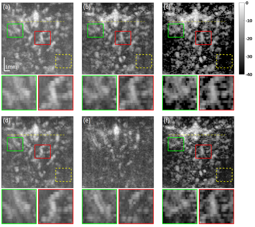
Rat data results. (a) SVD result. (b) Iterative result. (c) Unfolded result. (d) High-pass filter with high cut-off frequency. (e) High-pass filter with low cut-off frequency. (f) ResNet results.

Conclusions
- The authors proposed an RPCA decomposition of the tissue/blood separation problem in contrast-enhanced ultrasound imaging to exploit both spatial and temporal patterns.
- They first used an iterative resolution of the problem that outperformed classic methods such as SVD.
- They then proposed to unfold the iterative resolution into a deep neural network, that achieved better and faster results.
- They found that the unfolded method outperformed a ResNet but was slower to execute. They attributed this to the SVD computation time.