Shape-Aware Organ Segmentation by Predicting Signed Distance Maps
Highlights
- The goal of the paper is to improve organ segmentation results by predicting a Signed Distance Map (SDM) and a segmentation map jointly
- The contributions of the paper include a 3D-UNet-based backbone, a SDM learning model and a regression loss.
Introduction
The authors study the case of organ segmentation. Methods using CNNs (2D and 3D) output segmentation maps for which the anatomical shapes of the organs are not preserved. As illustrated in Figure 1, the maps also show a lack of smoothness, which requires a post-processing.

Figure 1: Hippocampus segmentation with (a) ground-truth, (b) predicted without SDM and (c) predicted with SDM
To solve these problems, the idea of the paper, is to have a supervision not only on the segmentation map but also on the SDM.
What is the SDM?
For each point in space (here, for each voxel), the signed distance map gives the distance between the point and the closest boundary of the target organ. The sign of the value is \(<0\) if the point is located inside the organ, \(>0\) if the point is located outside the organ and \(=0\) if it belongs to the surface of the organ. It is a continuous and implicit way to represent a shape.
Small changes in the shape of an organ will have effect on a large part of the SDM, while the segmentation map will be only slightly impacted.
Method
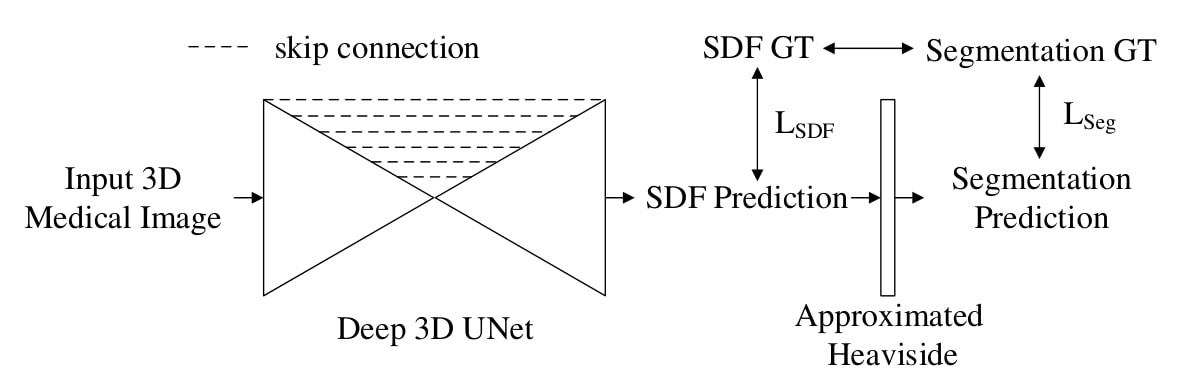
Figure 2: workflow proposed by the authors
Deep 3D UNet
The authors propose a backbone model based on 3D-UNet:
- 6 downsampling layers (more than a regular 3D UNet) with the largest receptive field being \(64^3\)
- Leaky-ReLU instead of ReLU
- Trilinear sampling instead of deconvolution
- Group normalization instead of batch normalization
- Dice loss
SDM learning
The ground truth SDMs are approximated from the segmentation maps using Danielsson Algorithm1, and normalized between \([-1;1]\).
The authors train a model which outputs a SDM. From this SDM, the segmentation map is computed with a Heaviside function. This function is the unit step function, defined as:
\[H(x)=\begin{cases} 1, x>0 \\ 0, x<0 \\ \end{cases}\]As the Heaviside function is not differentiable, they use an approximated version during training:
\[f(z)=\frac{1}{1+\exp{(-z\times k)}}\]where the larger k, the closer the approximation. They use \(k = 1500\).
During inference, they use the Heaviside not approximated.
Note: the authors also tried with two output branches but had better results with only one output
They also propose a regression loss based on the product, which penalizes the output SDM for having the wrong sign:
\[\mathcal{L}_{product}= -\sum_{t=1}^{C} \frac{y_t p_t}{y_t p_t+p_t^2+y_t^2}\]They use this loss, coupled with the L1-norm to get their SDM loss.
The total loss is then:
\[\mathcal{L}=\mathcal{L}_{Seg} + \lambda \mathcal{L}_{SDM} = \mathcal{L}_{Dice} + \lambda ( \mathcal{L}_{product} + \mathcal{L}_{1})\]with \(\lambda=10\).
Implementation
- Optimizer : Adam
- \(l_r= 5 \times 10^{− 4}\) initially and then decayed by factor of 0.8 for every 25 epochs
- 200 epochs for single-organ segmentation and 600 epochs for multi-organ segmentation
Results
Single Organ Segmentation
- Dataset: collected hippocampus segmentation CT scans with patients
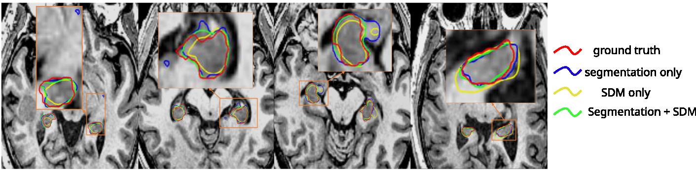
Figure 3: Qualitative segmentation comparison on the hippocampus testing set

Table 1: Quantitative comparison of segmentation models on the hippocampus dataset (the methods’ names correspond to the loss chosen)
- Compared to using only the segmentation map, the results have less false positives, and reduce the Hausdorff Distance (HD)
- Using only the SDM during training gives the smoothest contours
- Using the segmentation map and the SDM jointly gives more accurate results
Multi-organ Segmentation
- Dataset: MICCAI Head and Neck Auto Segmentation Challenge 2015 with CT images (38 for training and 10 for testing). The authors crop the volume around the head.
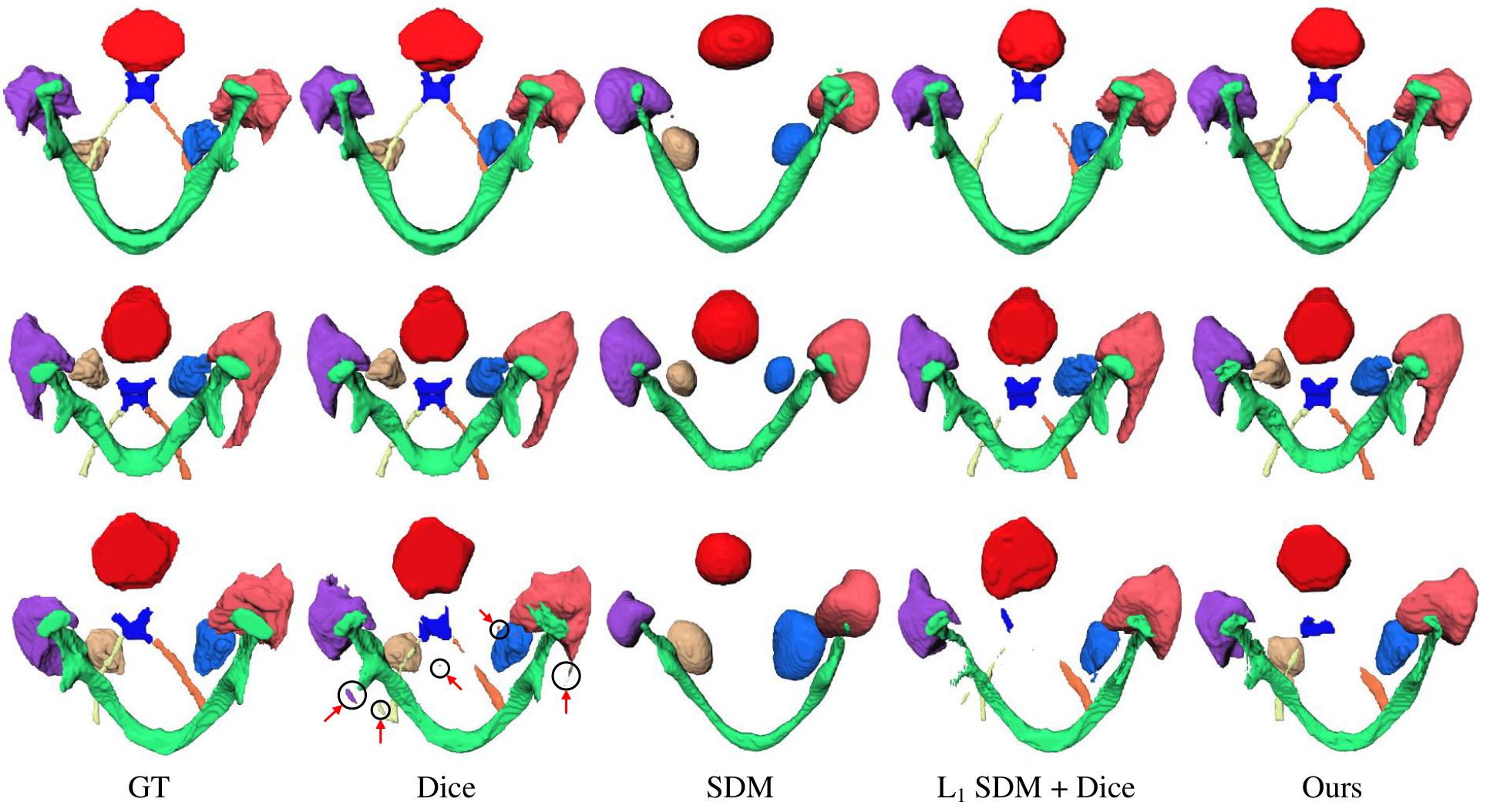
Figure 4: Qualitative results on the MICCAI 2015 Head and Neck segmentation testing set. Rows 1 and 2: results from Dice only training and from the joint training match with the groundtruth. Row 3: Dice result contains many isolated false positives. The proposed joint training model has smoother and better result in this case.
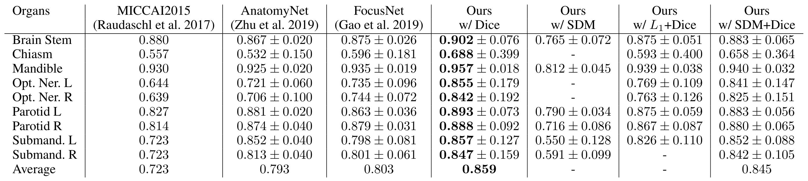
Table 2: Dice comparison on the MICCAI 2015 testing set

Table 3: comparison of proposed methods on the MICCAI 2015 testing set
Note: Average Symmetric Surface Distance (ASD or ASSD) is the average distance between boundary points from the predicted mask and from the ground truth mask.
- For the proposed backbone (Dice only), HD95 and Dice are improved for all organs but especially for small organs (chiasm, optic nerves)
- For the supervision with SDM only, the output is smoother but small organs are lost
- For the joint training, the model gives a more continuous shape compared to the segmentation only model. It also does not not lose organs contrary to the “SDM only” model. It has also the best averaged HD and ASD metrics.
The authors conclude that their regression loss based on the SDM stabilizes training and gives better results. However, there are still some difficulties for small organs segmentation in a multi-organ setting.
Conclusion
- The authors encourage the use of this method by adapting it to an existing network.