Github available here
Video of the presentation of the article by the author Antti Tarvainen here.

Highlights

Method : The mean teacher model averages model weigths, instead of label predictions like the Temporal Ensembling method. Allows for more accurate targets and faster feedback between the student and teacher models.
Performances : demonstrates enhanced performance on various datasets (SVHN, CIFAR-10, and ImageNet) when combined with residual networks. Achieves lower error rates and higher accuracy compared to Temporal Ensembling, even when trained with fewer labeled examples.
Scalability and applicability : Enables working on larger datasets, and training with fewer labeled examples.

Introduction

Limitations of deep learning models :

require large number of parameters and are prone to overfitting.
manual high quality labels for training data is expensive and time consuming.

Interest in semi-supervised learning to use the unlabeled data effectively.

→ focus on regularization methods in semi-supervised learning

Method

Applying noise and Ensembling method

Noise regularization

Add noise to the input or intermediate representations of a model
Helps learning abstract invariances
Pushes decision boundaries away from labeled data points

Limitations of noise regularization :

classification cost is undefined for unlabeled examples → not helpful in semi-supervised learning.

→ The \(\Gamma\) model aims to overcome this

The \(\Gamma\) model¹

Evaluates each data point with and without noise, and then applies a consistency cost between the two predictions.
It’s a student teacher model: the teacher generates targets, which are then used by itself as a student for learning

Limitations of \(\Gamma\) model :

the model itself generates targets, which may be incorrect
the cost of inconsistency outweighs that of misclassification, preventing the learning of new information
can lead to a confirmation bias

→ Confirmation bias can be mitigated by improving the targets. One way is illustrated with the \(\Pi\) model, selecting a different teacher model than the student model

NOTE : The authors mention another way “to choose the perturbation of the representations carefully instead of barely applying additive or multiplicative noise” which is the subject of another paper by Miyato et al. (2017)² that will be refered as VAT+EntMin latter.

The \(\Pi\) model³

noise is added to the model during inference
results in a “noisy teacher” that can provide more accurate targets.

→ The \(\Pi\) model can be further improved by Temporal Ensembling (TE)

Temporal Ensembling (TE)

exponential moving average (EMA) prediction for each training example is formed by combining the current version of the model’s predictions with the predictions made by earlier versions of the model that evaluated the same example.
improves the quality of the prediction
better results when those predictions are used as the teacher predictions

Limitation of Temporal Ensembling :

Each target (prediction) is updated only once per training epoch.
The learned information is incorporated into the training process at a relatively slow pace.
The larger the dataset, the longer it takes for the updates to span the entire dataset.

→ The authors propose the Mean Teacher model that averages model weights, instead of predictions like TE, to improve performances of semi-supervised model.

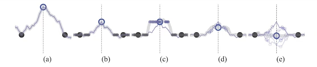
A sketch of a binary classification task with two labeled examples (large black dots) and one unlabeled example, demonstrating how the choice of the unlabeled target (blue circle) affects the fitted function (gray curve).

(a) A model with no regularization
→ free to fit any function that predicts the labeled training examples well
(b) A model trained with noisy labeled data (small dots)
→ consistent predictions around labeled data points
(c) The teacher model (gray curve) is first fitted to the labeled examples, and then left unchanged during the training of the student model. The student model has noise, the teacher doesn’t.
→ Consistency to noise around unlabeled examples provides additional smoothing. Used by the \(\Gamma\) model.
(d) Noise on the teacher model reduces the bias of the targets without additional training. Average of multiple predictions by the teacher.
→ The expected direction of stochastic gradient descent is towards the mean (large blue circle) of individual noisy targets (small blue circles). Used by the \(\Pi\) model.
(e) Ensemble model
→ gives an even better expected target. Both Temporal Ensembling and the Mean Teacher method use this approach

Mean Teacher

The Mean Teacher is an average of consecutive student models.

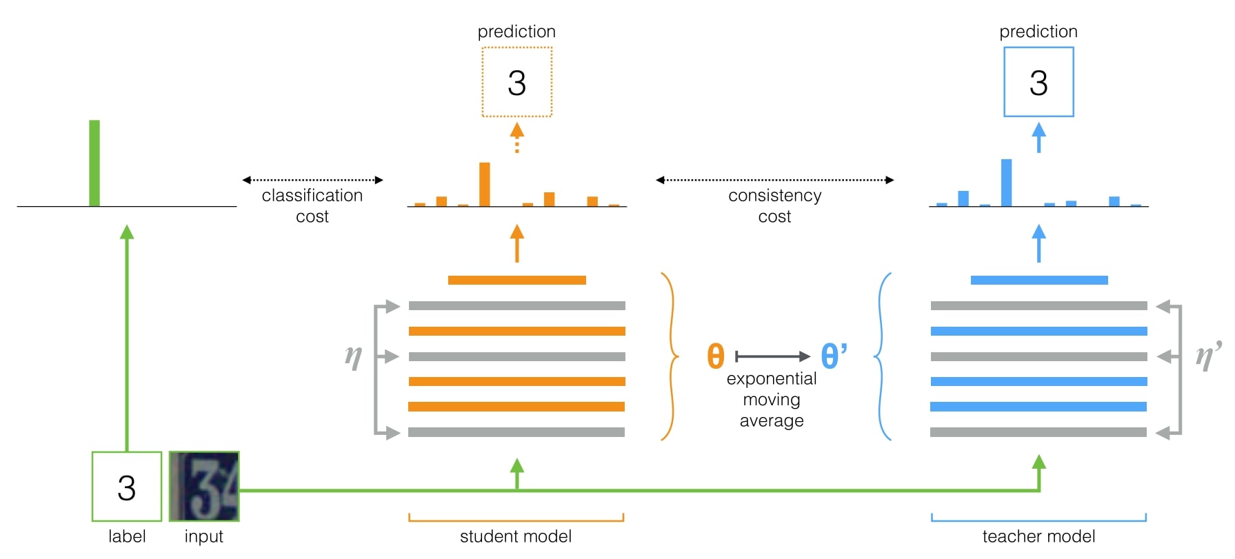
Both the student and the teacher model evaluate the input applying noise (η, η’)
The softmax output is compared with one-hot label using classification cost for the student model and consistency cost for the teacher
The teacher model weights are updated using the EMA weights of the student model.
Both predictions can be used but the teacher prediction is more likely to be correct
No classification cost is applied when it is a training step with unlabeled example.

Consistency cost

With \(J\) the consistency cost, as the expected distance between the prediction of the student model (with weights \(θ\) and noise \(η\)) and the prediction of the teacher model (with weights \(θ'\) and noise \(η'\)) :

\[J(θ) = \underset{x,η',η}{E} [ || f (x, θ', η') - f (x, θ, η) ||^2 ]\]

Mean squared error is applied to the distance to get the consistency cost. The weight of this consistency loss changes during training: it ramps up from 0 to its final value during the first 80 epochs. → Initially ignoring it and then gradually introducing more and more consistency.

Difference between the \(\Pi\) model, Temporal Ensembling, and Mean teacher

How the teacher predictions are generated :
- \(\Pi\) model : \(θ' = θ\)
- TE : approximates \(f (x, θ', η')\) with a weighted average of successive predictions
- Mean Teacher defines \(\underset{t}{θ'}\) at training step as the EMA of successive \(\theta\) weights, where \(\alpha\) is a smoothing coefficient hyperparameter :

\[\underset{t}{θ'} = α \underset{t-1}{θ'} + (1 - α)\underset{t}{θ}\]

Weights \(\theta'\) :
- \(\Pi\) model : applies training to it
- TE and Mean teacher : treat it as a constant with regards to optimization

Type of noise

Random translations and horizontal flips of the input images
Gaussian noise on the input layer
Dropout applied within the network

Loss

Student : cross-entropy loss
Teacher : consistency loss multiplied by an importance weight

Data

Street View House Numbers (SVHN) :

32x32 pixel RGB images belonging to ten different classes
close-up of a house number, and the class represents the identity of the digit at the center.
73,257 training samples and 26,032 test samples.

CIFAR-10 :

32x32 pixel RGB images belonging to ten different classes
natural image belonging to a class such as horses, cats, cars and airplanes etc
50,000 training samples and 10,000 test samples.

Results

Comparisons with the state-of-the-art methods:

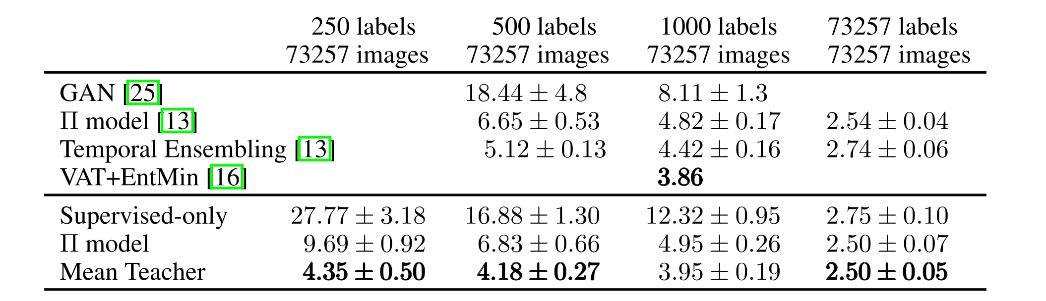
Mean Teacher improves test accuracy over the \(\Pi\) model and Temporal Ensembling on semi-supervised SVHN tasks.

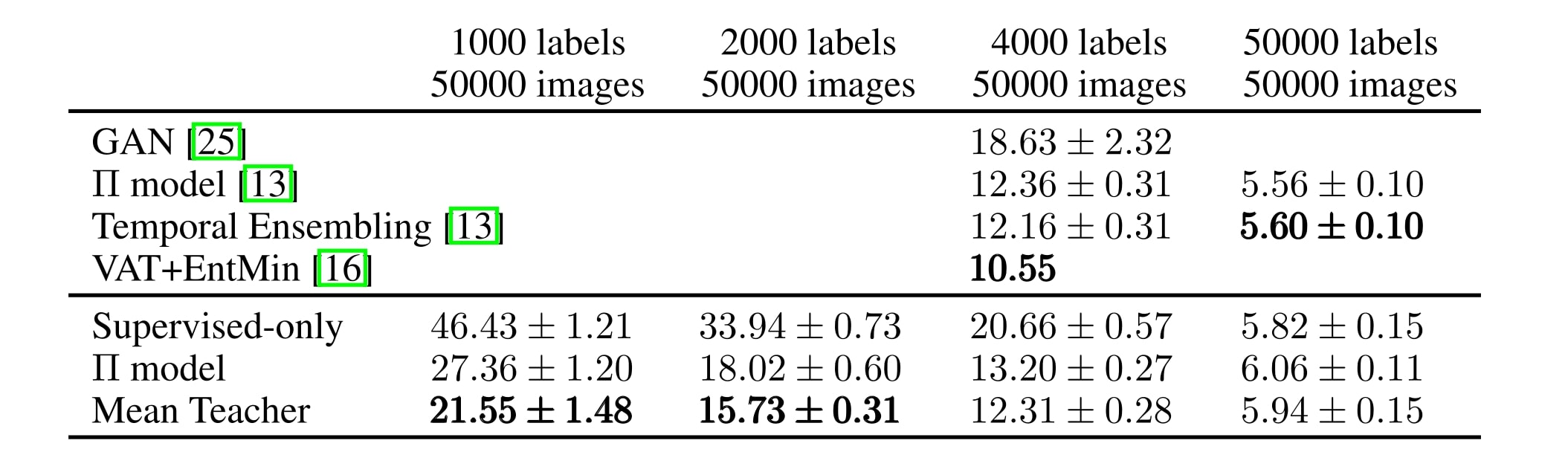
Mean Teacher also improves results on CIFAR-10 over our baseline \(\Pi\) model.

NOTE : The Virtual Adversarial Training (VAT) by Miyato et al. 2017² performs even better than Mean Teacher on the 1000-label SVHN and the 4000-label CIFAR-10. VAT and Mean Teacher are complimentary approaches.
→ Their combination may yield better accuracy than either of them alone.

Error percentage over 10 runs on SVHN with extra unlabeled training data:

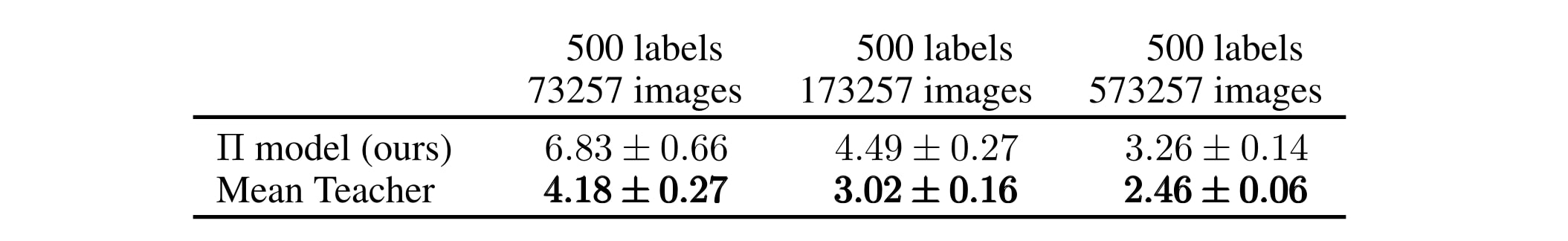
Effect of using mean teacher:

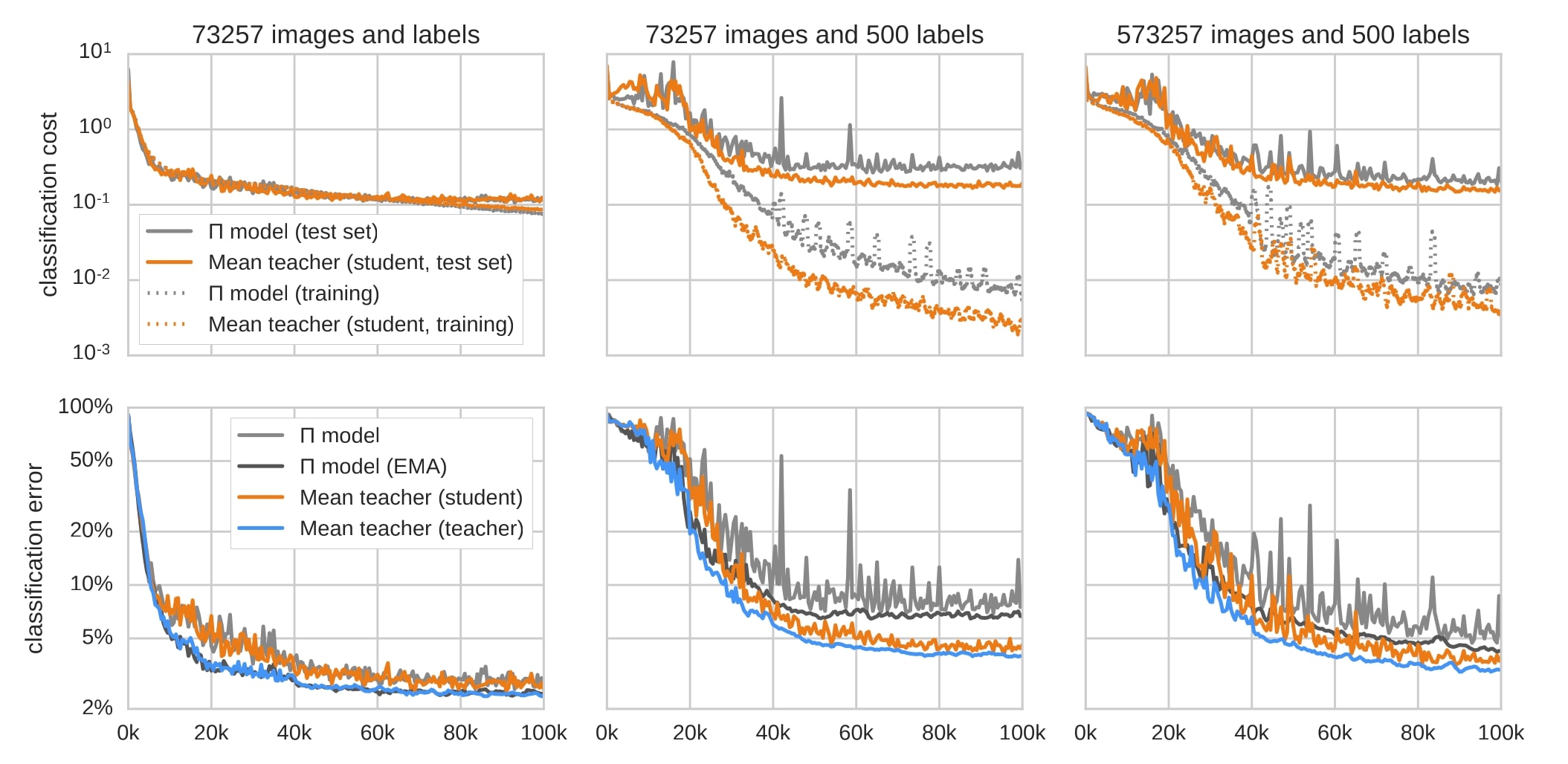
The EMA-weighted models (blue and dark gray curves in the bottom row) give more accurate predictions than the bare student models (orange and light gray) after an initial period.

→ EMA-weighted model as the teacher improves results in the semi-supervised settings
When using 500 labels Mean Teacher learns faster, and continues learning after the \(\Pi\) model stops improving.

→ Mean Teacher uses unlabeled training data more efficiently than the \(\Pi\) model
In the all-labeled case, Mean Teacher and the \(\Pi\) model behave identically. With 500k extra unlabeled examples \(\Pi\) model keeps improving for longer.

→ Mean Teacher learns faster, and eventually converges to a better result, but the sheer amount of data appears to offset \(\Pi\) model’s worse predictions.

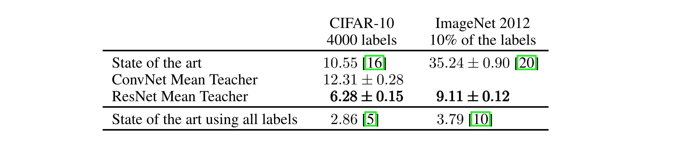
Mean Teacher with residual networks on CIFAR-10 and ImageNet

Checking if the methods scales to more natural images on ImageNet with 10% of the labels :

Conclusions

Advantages over Temporal Ensembling :

more accurate target labels, which enables faster feedback loop between the student and the teacher model
scales to large datasets and online learning.

To conclude :

The success of consistency regularization depends on the quality of teacher-generated targets.
Mean Teacher and Virtual Adversarial Training represent two ways of exploiting this principle.

→ Their combination may yield even better targets.

Mean teachers are better role models: Weight-averaged consistency targets improve semi-supervised deep learning results

Highlights

Introduction

Method