Towards Robust Interpretability with Self-Explaining Neural Networks
Useful links: GitHub repository (PyTorch), submission process
Highlights
- Post-hoc interpretability methods are not always faithful in regard to models’ predictions and their explanations aren’t robust to small perturbations of the input1
- The authors propose a class of intrinsically interpretable neural networks models which are as interpretable as linear regression
Introduction
- Most interpretability methods are post-hoc, explaining the model after its training
- But their explanations lack stability, small changes to the input can lead to different (or even contradictory) explanations for similar predictions
- Linear models are considered to be interpretable, which is the starting point of this paper
Self-Explaining Neural Networks models
Intuition
Linear models are considered interpretable for 3 reasons:
- Input features are clearly grounded (arising from empirical measurements)
- Each parameter \(\theta_i\) provides direct positive/negative contribution of each feature for the prediction
- Features impact can be easily differentiated because of the sum
Formalization
Supervised problem: linear regression:
\[f(x) = \sum_i^n \theta_i x_i + \theta_0 \tag{1}\]To improve the modeling power, the coefficients themselves can depend on the input \(x\):
\[f(x) = \theta(x)^T x \tag{2}\]Locally linear
The function \(\theta(\cdot)\) can be anything from a simple model to deep neural networks. But to maintain a decent level of interpretability, \(\theta(x)\) and \(\theta(x')\) should not differ significantly for close inputs \(x\) and \(x'\), \(\theta(\cdot)\) needs to be stable. More precisely:
So the model acts locally, around each \(x_0\), as a linear model with a vector of stable coefficients \(\theta(x_0)\)
Concepts
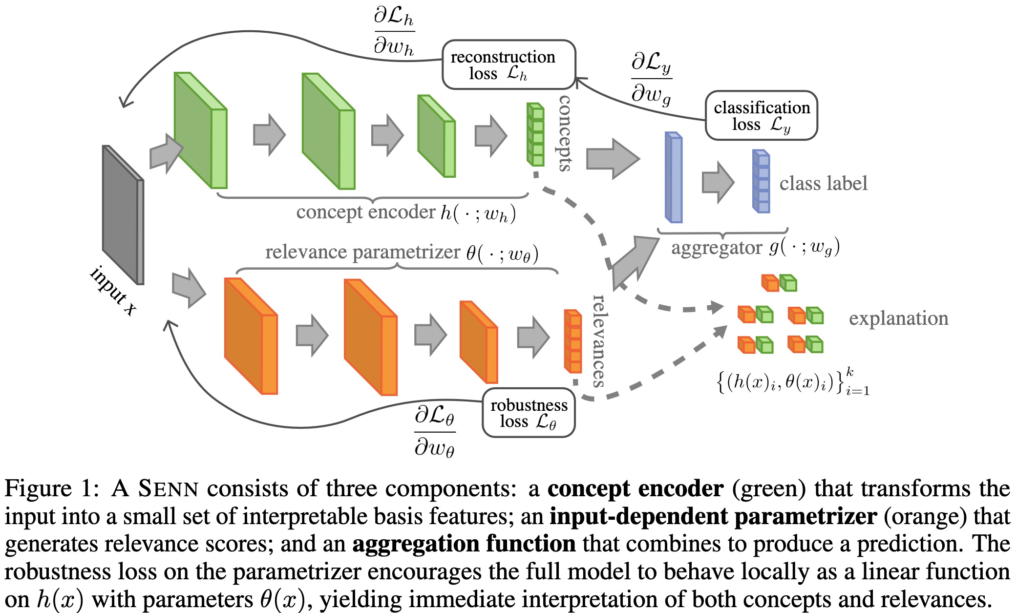
Then, explanations can also be considered in terms of higher order features, or concepts, derived from the input, like a function \(h(x) : \mathcal{X} \rightarrow \mathcal{Z}\) where \(\mathcal{Z}\) is some space of interpretable concepts. The model thus becomes:
General model
And finally, the aggregation function, e.g. the sum, can also be replaced by a more general form. This general aggregation function would need specific properties like permutation invariance or the preservation of relative magnitude of the impact of the relevance values \(\theta(x)_i\). This would result in a model of the following form:
Proposed stability loss
Now, the stability, or slow variation, of \(\theta(\cdot)\) should be pursued in regards to \(h(x)\) and not \(x\). Thus, the objective is now to enforce \(\theta(x_0) \approx \nabla_z f\) with \(z = h(x)\). Using the chain rule, it implies the following loss for \(\theta\):
This results in the following loss for the model to optimize:
\[\mathcal{L}_y(f(x), y) + \lambda \mathcal{L}_\theta(f) + \xi \mathcal{L}_h(x, \hat{x}) \tag{3}\]Experiments
Interpretable models need to be evaluated in term of accuracy on the prediction task and how the produced explanations are perceived by explainability recipient, ie, users. So the proposed model is compared with non-interpretable counterparts and 3 criteria are defined to evaluate provided explanations:
- Explicitness/Intelligibility: are the explanations immediately understandable?
- Faithfulness: are relevance scores indicative of “true” importance?
- Stability: how consistent are explanations for similar/neighboring examples?
Datasets used
- MNIST & CIFAR10
- Images classification
- 32x32 & 32x32x3
- Several datasets from UCI Machine Learning Repository
- Regression, classification, segmentation tasks
- Data types are numerical, categories, images, …
- Propublica’s COMPAS Recidivism Risk Score
- COMPAS is a closed-source model used by USA DoJ to evaluate probability of recidivism
- Dataset consists of results from the score, often used to evaluate fairness of predictive algorithms
Architectures details and accuracy results
The authors do not detail their predictive performances on previously mentioned datasets, only that the proposed models are
on-par with their non-modular, non interpretable counterparts.
They just precise achieving less than 1.3% error rate on MNIST test set or an accuracy of 78.56% on CIFAR10 test set, which is “on par for models of that size trained with some regularization method”.
For each task, they used different architectures for the sub-branches \(h (\cdot)\) and \(\theta (\cdot)\) of the SENN model. FC stands for Fully connected layer, and CL for Convolutional layer. The multiplicative constant 10 in the final layer of the \(\theta\) function for both MNIST and CIFAR10 corresponds to the number of classes. In all cases, the training occurred using Adam optimizer with a learning rate \(l = 2 \times 10^{-4}\), and the sparsity of learned \(h(\cdot)\) was enforced through \(\xi = 2 \times 10^{-5}\).

Intelligibility
Explanations of this model are to be understood relative to the concepts defined. Here, they propose to retrieve examples of the dataset which maximally activate specific concepts.

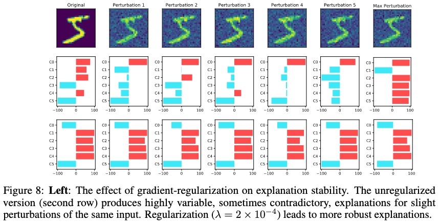
Stability
Empiric tests show low robustness of interpretability methods to local perturbations of the input. Small changes in the input produce visible modifications of the explanations
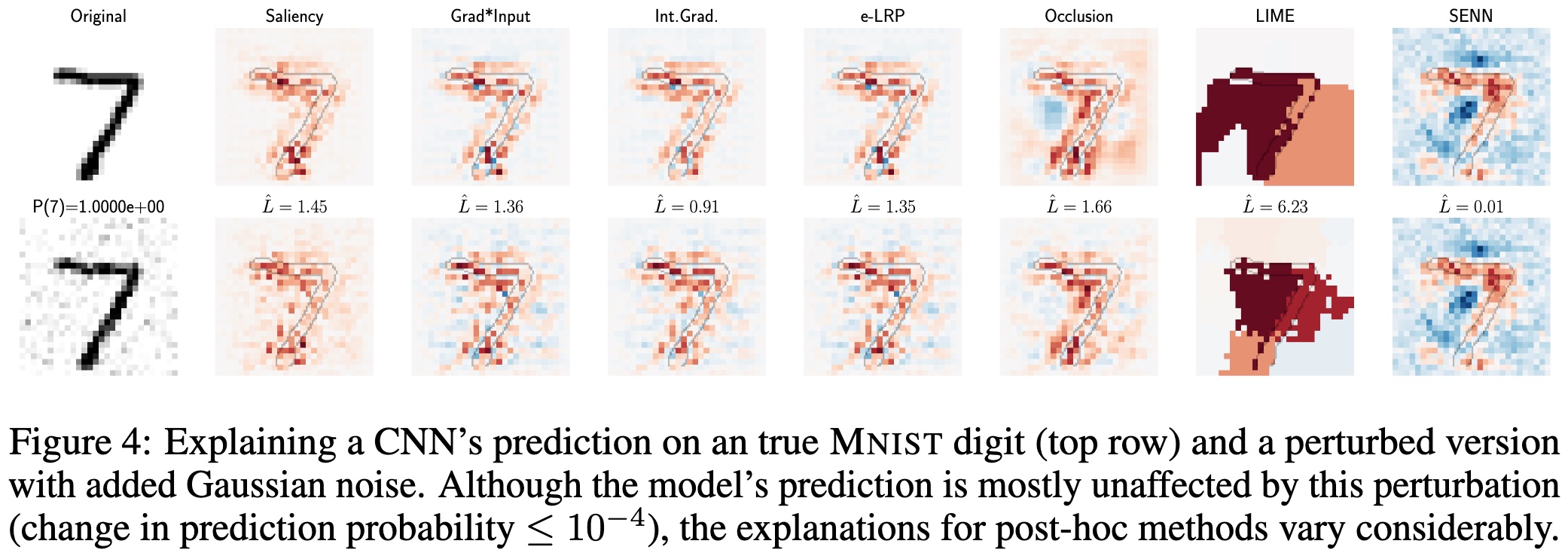
The Self-Explaining Neural Network model is less subject to adverse effects of input perturbation on explanations stability.
Limitations
- No details on model performances, even in supplementary materials
- Definition of interpretable concepts is a problem in itself
- The final prediction is more explainable, but the intermediate steps are not: the concept encoder and relevance parametrizer are still complete black-boxes