NISF: Neural Implicit Segmentation Functions
Notes
- Link to the code here
Highlights
- The goal of the paper is to perform segmentation using neural implicit functions to avoid limitations of CNNs.
- The authors propose an auto-decoder network and apply their method to cardiac MRI segmentation.
Introduction
CNNs have produced satisfying results for segmentation of medical images but still face some limitations including the difficulty to handle partial data, or their high computational cost.
The authors propose a new type of model based on neural implicit functions (NIF) to perform segmentation.
What are NIFs? NIFs are models which map a signal (for example: image intensity, segmentation) from a coordinate space.
The authors propose a model NISF (Neural Implicit Segmentation Functions) that use NIFs. This model produces a segmentation as well as interpolates the results to unseen areas of an image, at an arbitrary resolution.
Method

Figure 1: workflow proposed by the authors
Architecture
From an input {single sample coordinate + latent vector}, NISF outputs {image intensity + segmentation label}.
The network consists of an MLP with 8 residual layers of 128 hidden units each. This MLP jointly learns two functions:
- a reconstruction function \(f_\phi\) that gives the image intensity \(i_c\) for any queried coordinate,
- a segmentation function \(f_\theta\) that gives the segmentation probability of each label \(s_c\) for said coordinate.
The authors use Gabor wavelet activation function, combined with ReLU or sinusoidal activation function.
Prior training
The presented method uses an auto-decoder that simultaneously optimizes the weights of the network, as well as a latent vector \(h_j\) representing each subject \(j\).
Therefore, during training, the network learns a shared prior \(\mathcal{H}\) over all subjects.
The steps are:
- initialize H, the matrix of all latent codes from the population
- process all voxels from a 3D volume in parallel
Loss function:
- image reconstruction: binary cross-entropy loss (BCE)
- image segmentation: BCE + Dice loss
- L2 regularization for both tasks
Note: the authors found that the weighting factor \(\alpha=10\) improves performances
Inference
Following the auto-decoder workflow, during inference, the weights of the MLP are frozen. The latent vector \(h_j\) is thus optimized using the knowledge of the pair coordinate-image \((c,i_c)\). The authors assume that optimizing the latent code on intensity values will also produce a satisfying segmentation.
The steps are:
- initialize the subject latent code \(h\)
- optimize \(h\) on the image intensities
Loss function:
- image reconstruction: BCE + L2
Implementation
- Optimizer: Adam
- Training time: 9 days (1000 epochs)
- Inference time: 3 to 7 min
- Latent code: 128 learnable parameters
Data
- UK Biobank short-axis cardiac MRI
- 1150 subjects (data split: 1000/50/100)
- Preprocessing: intensity normalization
- Ground truth segmentation: synthetic segmentation produced with a state-of-the-art CNN by (Bai et al.)1
- Segmentation label: left ventricule (LV) blood pool, LV myocardium, right ventricle (RV) blood pool
Results
Figure 2 shows overfitting of the latent code to the reconstruction: to have the optimal code for segmentation, early-stopping is needed.
 Figure 2: Segmentation Dice trend during a subject’s inference
Visual results from Figure 3 show the need to learn the shared prior, which enables better reconstruction and segmentation performances.
 Figure 3: Inference-time segmentation and image reconstruction at various stages of the prior’s training process
The results after 672 optimization steps (optimal number based on the DICE scores from validation set) are presented in Table 1.
 Table 1: Class Dice scores for the 100 subject test dataset
The Figure 4 shows the generalization capabilities of the subject prior: the latent code is optimized only on a subset of the original volume. The authors compare the ground-truth held-out slices with the reconstructed image and their segmentations. They show that the model finds a plausible reconstruction and segmentation, even for the RV in the basal slices which is more challenging to annotate.
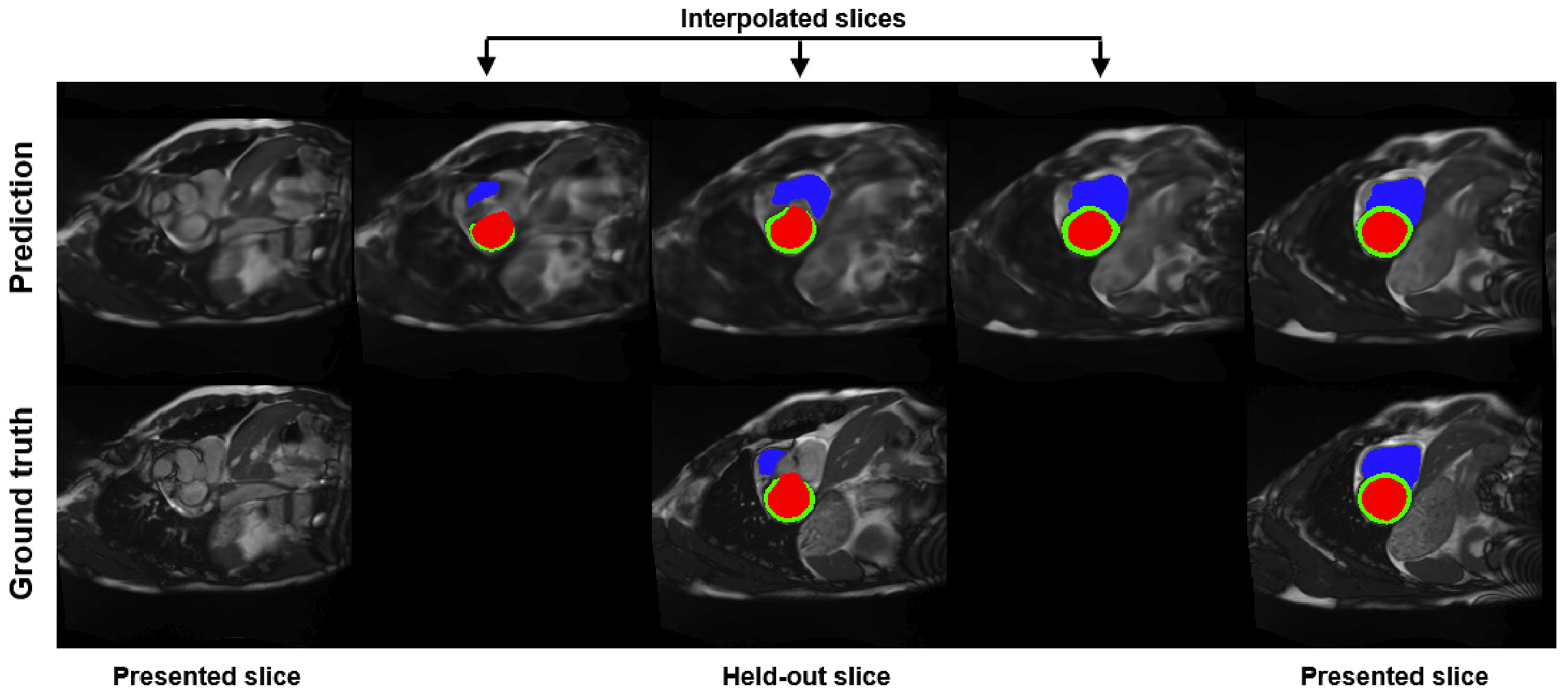 Figure 4: Interpolation predictions for a held-out basal slice
Conclusion
NISF can
- produce segmentations at an arbitrary resolution
- make predictions in unseen areas of the volume.
A strength of NISF is that it can be trained on partial/sparse data and is not affected by changes in image resolution.