Image as Set of Points

Highlights

• The authors propose Context Clusters (CoCs) which is a new paradigm for visual representations where images are seen as a set of unorganized points.
• Even though they don’t achieve state-of-the-art performances, they are still on par with recent convolutional and transformer-based visual backbones.
• CoCs have some good properties such as generalization to different data domains (point clouds, RGBD images, etc.) and good interpretability.
• Code is available on this GitHub repo.

 

Context Clusters

To translate an image to a set of points, an input image \(\textbf{I} \in \mathbb{R}^{3 \times w \times h}\) is changed to an augmented collection of points (pixels) \(\textbf{P} \in \mathbb{R}^{5 \times n}\) with \(n = w \times h\) and where each pixel \(\textbf{I}_{i,j}\) has its RGB channel values enhanced with its 2D coordinates \([\frac{i}{w} - 0.5 ; \frac{j}{h} - 0.5]\) to give a vector of 5 numbers.

Then, the features are extracted from this set of points with a succession of Points Reducers and Context Clusters blocks (Figure 1). As one of the goals of the model is to be plugged as a backbone feature extractor into more complex architectures, it copies the global architecture and intermediate/final output sizes of standard CNN and transformer-based backbones such as ResNet and ViTs. In particular, at each stage, the number of points is set so that it can be turned back into a square 2D image.

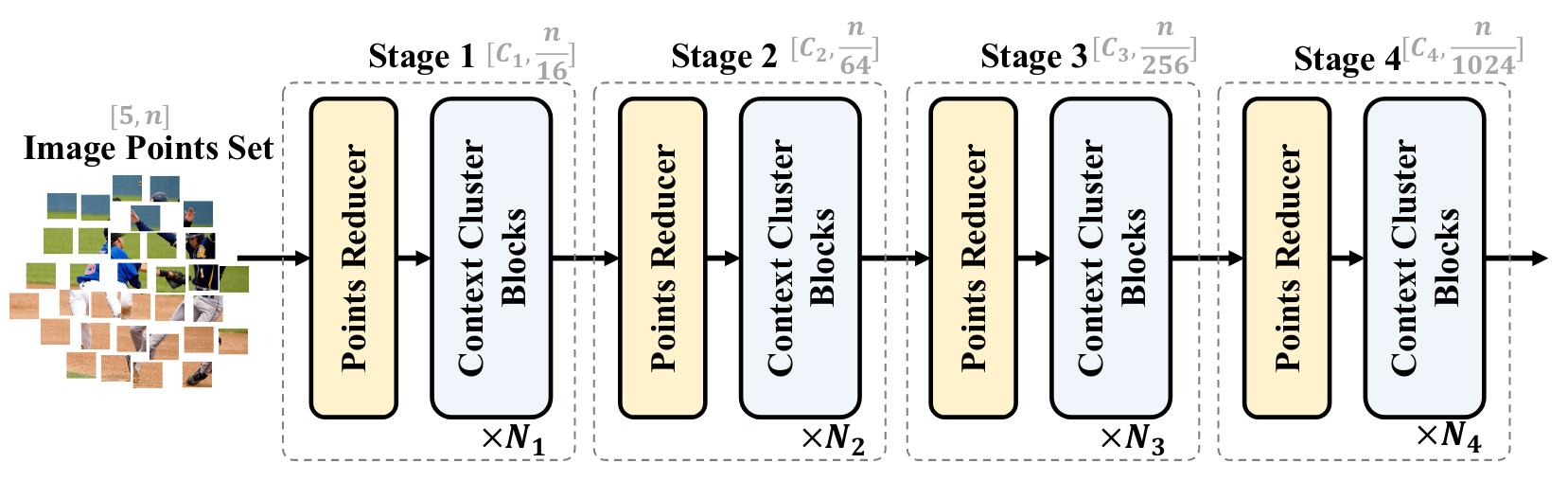
Figure 1. High-level overview of Context Cluster architecture with four stages.

Point reduction.   The point reduction operation is done by placing evenly spaced anchors in the image. The feature of the resulting point is obtained after a linear projection of the concatenated features of the k nearest points (Figure 2). While k can be any number, if it is properly set (for instance 4, 9 or 16), this operation can be done with a standard convolution, which is what is done by the authors. This mechanism is the same as the initial patch embedding in ViTs.

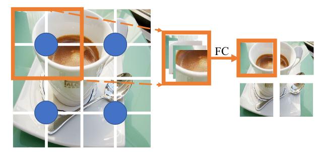
Figure 2. Illustration of anchors for point reduction. The blue points are the anchors and the red square shows the points that are aggregated for the top-left anchor.

Context Cluster Operation

The main proposal of the authors is the context cluster block, which will be described in details in this section. In each block, three main operations are done : context clustering, feature aggregation and feature dispatching

Context clustering.   Given a set of \(n\) feature points of size \(d\), \(\textbf{P} \in \mathbb{R}^{n \times d}\), they are linearly projected into a smaller space \(\textbf{P}_S\) for computational purposes. Then, similarly to point reduction, \(c\) centers are evenly distributed in space and the center feature is computed as the average of the \(k\) nearest points of each center.

Then, the pair-wise cosine similarity between the center and each feature points \(\textbf{P}_S\) is computed and gives a matrix \(\textbf{S} \in \mathbb{R}^{c \times n}\). Note that it is implicitly both a similarity between points’ distances and features. Finally, each point is assigned to its most similar center (unique association), resulting in \(c\) clusters (Figure 3), that have a different number of points (and may also be empty).

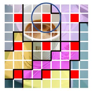
Figure 3. Illustration of the computation of the center features. The red squares are the centers, the blue circle shows the features that are averaged for the top center, and the color palette shows the clusters of points associated with each center.

 

Feature aggregating.   Given a cluster \(c\) with \(m\) points, the points are mapped to a high-dimension value space \(\textbf{P}_v \in \mathbb{R}^{m \times d'}\). A center \(v_c\) is also computed in the value space like it is done at the clustering step.

In practice, the dimension of the value space is set to be equal to d’ so this step can be skipped.

The aggregated feature \(g \in \mathbb{R}^{d'}\) of the cluster \(c\) is computed as :

\[g = \frac{1}{C} \left( v_c + \sum_{i=1}^{m} \text{sig}(\alpha s_i + \beta) \ast v_i \right)\]

with \(C = 1 + \sum_{i=1}^m \text{sig} (\alpha s_i \ast \beta)\).

\(v_i\) is th \(i\)-th point in \(\textbf{P}_v\), \(\alpha\) and \(\beta\) are learnt scalars and \(\text{sig}(\cdot)\) is the sigmoïd function. \(v_c\) and \(C\) are added for numerical stability.

Feature dispatching.   Once the aggregated feature \(g\) has been computed inside a cluster, it is adaptively dispatched to each point in a cluster based on the similarity. This allows pixels inside a cluster to interact. Each point \(p_i\) is updated as follows :

\[p_i ' = p_i + \text{FC}(\text{sig} (\alpha s_i + \beta) \ast g )\]

where \(\text{FC}\) is a fully-connected layer to get back to the original dimension \(d\) from the value-space dimension \(d'\)

A schematic view of a context cluster block is given is Figure 4.

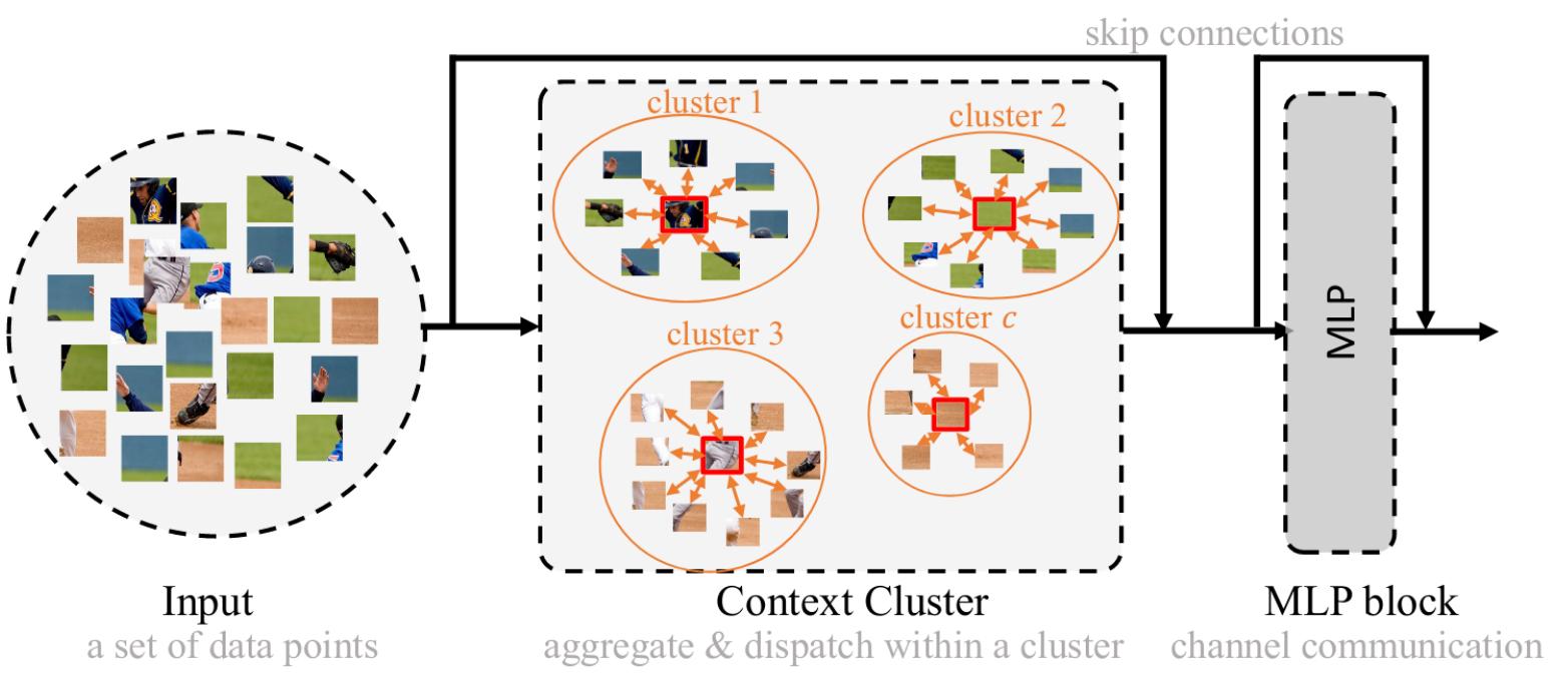
Figure 4. Overview of a Context Cluster block.

 

Choices for computation time improving

Multi-head design.   Like in ViTs, the authors use a multi-head design in the context cluster. The output of all the heads are concatenated and fused by a fully-connected layer.

Region splitting.   If no restriction is set when associating the points with the centers, the time complexity to calculate the feature similarity is \(O(ncd)\) (with \(n = h \times w\)), which is quadratic relative to the number of points in the image. As it is too computationally demanding, the same technique as in SwinTransformer is done, that is to say splitting the points into several local regions.. If the number of regions is set to \(r\), the time complexity is lowered to \(O(r\frac{n}{r}\frac{c}{r}d)\). This obviously results in a trade-off between time complexity gain and limitation of the receptive field. In practice, the parameter \(r\) is set so that the clusters are computed in a \(7 \times 7\) window.

 

Results

The architecture is evaluated on several datasets for image classification, point cloud classification, object detection, instance segmentation and semantic segmentation tasks. Even though the performances do not reach that of the best state-of-the-art models such as ConvNeXt or DaViT, they are on par with other recent CNN and transformer-based backbones.

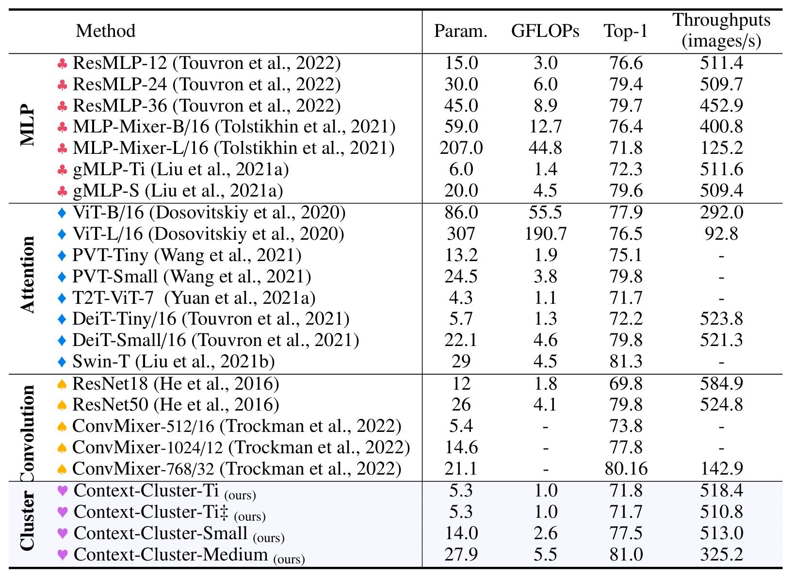
Table 1. Results on several backbones on ImageNet-1k classification benchmark.

An important result shown in Table 1 is the two first lines of the cluster-based methods. \(\text{Context-Cluster-Ti } \ddagger\) has the same architecture as the other models execpt that the image is split into much fewer local regions for clustering operations. The small difference of performance between this version of the model and \(\text{Context-Cluster-Ti }\) is an argument in favor of the region-splitting strategy.

 

Context clusters can be adapted and plugged into point cloud classification networks such as PointMLP or used with Mask-RCNN for object detection and instance segmentation.

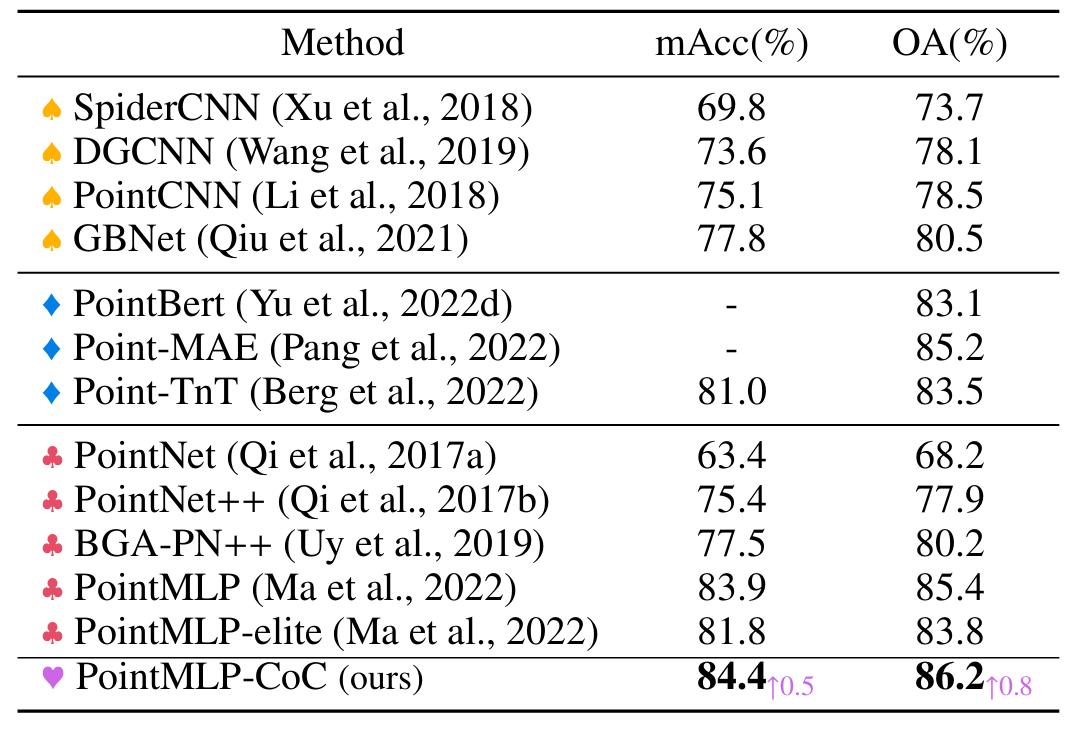
Table 2. Classification results on ScanObjectNN.

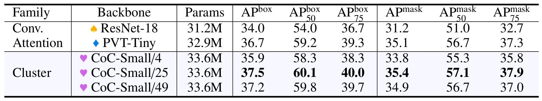
Table 3. COCO object detection and instance segmentation results using Mask-RCNN .

 

A nice property of treating images as sets of points and clustering them is that it is much easier to see which pixels interact compared to CNN or ViTs for which complex activation maps have to be computed to get analogous visualizations.

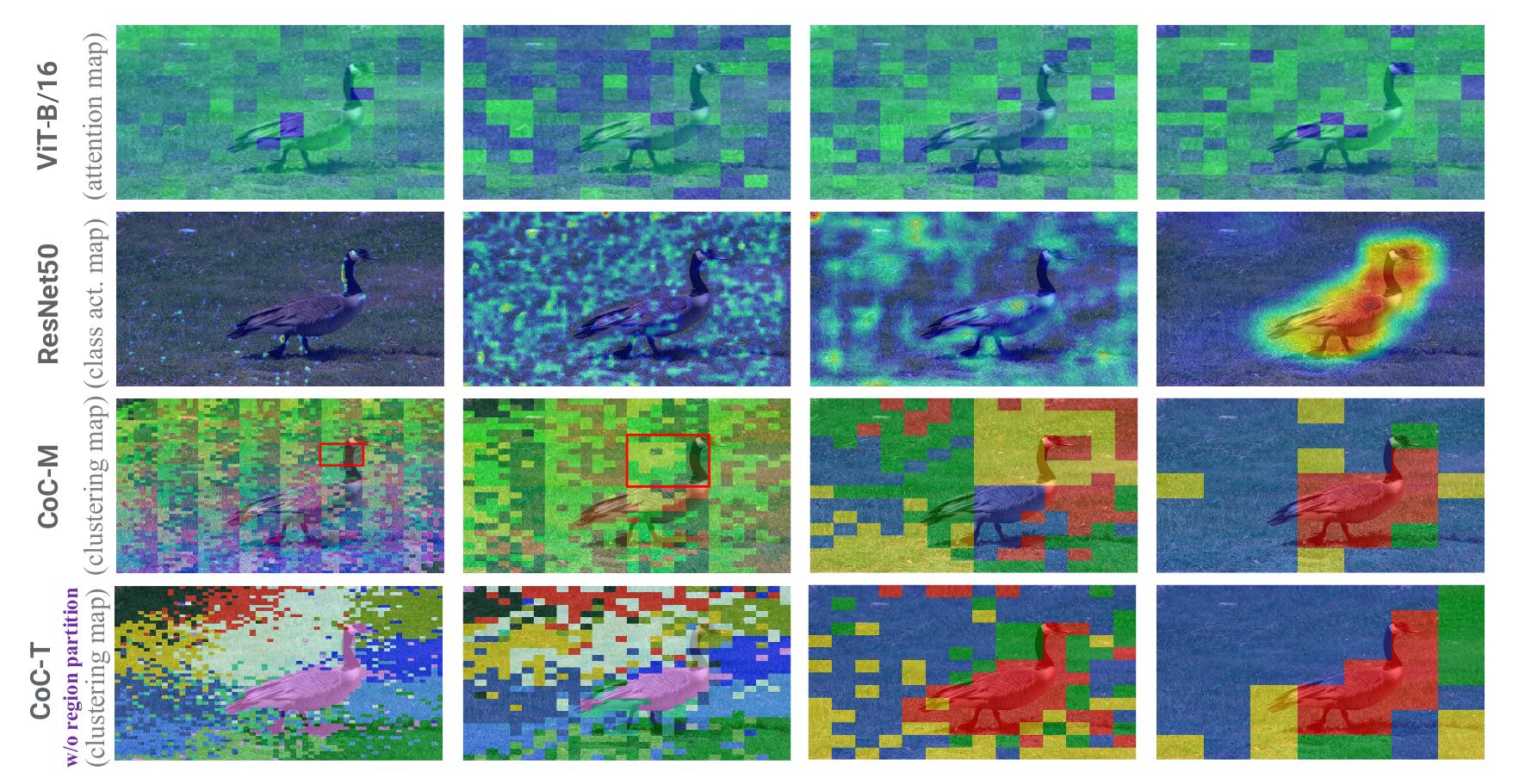
Figure 5. Visualization of activation map, class activation map and clustering map for various models and at different stages.

Conclusion

See highlights, you know how it works.