Tweedie's formula for self-supervised denoising without clean images

Highlights

• Denoising without requiring clean / noisy pairs: only noisy samples ! Making it very useful for practical applications
• One (!) denoiser for any type of noise: Gaussian, Poisson, Gamma
• Can even handle blind denoising

About the authors

Both authors come from KAIST, one of the biggest research lab in South Korea. The second author, Jong Chul Ye is focusing his research on using Deep Learning in medical imaging. He’s very famous for his recent series of papers on diffusion models applied to inverse problems with Hyungjin Chung, which were then very broadly applied to medical imaging. If you see diffusion models used to improve the image quality / reconstruction of any modality, be it Ultrasound, MRI, CT or PET, it is probably an adaptation of his work. You can find an interesting review documenting these applications of diffusion models here: https://academic.oup.com/bjrai/article/1/1/ubae013/7745314.

Motivations

Denoising is one of the pillars of image restoration. If we take the general inverse problem formulation:

$$y = Ax + \epsilon$$

with $\epsilon \sim \mathcal{N}(0, \sigma^2)$ and $A$ a degradation operator (for instance blur), denoising can then be considered as the easiest situation corresponding to the case $A = \mathrm{Id}$. However, denoising is still not considered an entirely solved problem. Most denoising techniques rely on training a UNet with clean and noisy pairs, which provides very good performances on Gaussian noise ¹.

Of course, finding such clean and noisy pairs is costly, or even impossible in many cases. For instance in medical imaging, one may consider doing longer acquisitions to reduce the noise in the image, and produce a “clean” image. But having exactly the same noisy version of the image is then very challenging, as the acquisition setting can’t be exactly reproduced.

It is then interesting to consider the setting where only noisy data is available for training.

Reminders

An important aspect of Gaussian denoisers is that they learn the underlying score function of a probability distribution. This fact has been extensively used in Diffusion Models to generate new data from these distributions.

The score function

Let us take a probability distribution $p(x)$, which represents the distribution of dog images. The score function is then just the gradient of the log of this distribution $\nabla \log p(x)$.

This quantity is very useful for two reasons:

• it eliminates the normalizing constant of $p(x)$ which is often impossible to estimate
• it acts as a compass pointing towards regions of high probability, meaning regions of the space where data coming from $p(x)$ is most likely to be located

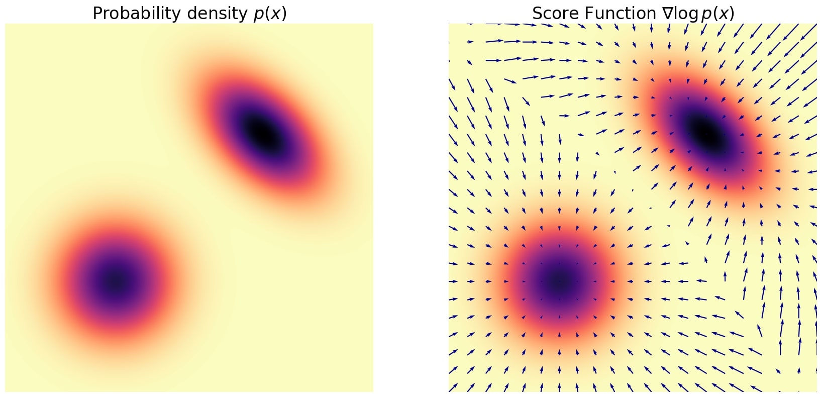
Figure 1. A Gaussian mixture and its exact score function.

 

Tweedies’ formula

Training any statistical model to remove Gaussian noise relates to the score function by Tweedie’s formula ²:

$$\mathbb{E} \left[ x \mid y \right] = y + \sigma^2 \nabla \log p(y)$$

where $y \sim \mathcal{N}(0, \sigma^2)$. The link between this formula and our good old autoencoders is that when we trained an autoencoder to remove Gaussian noise with the Mean Squared Error (MSE), we actually estimate the posterior mean $\mathbb{E} \left[ x \mid y \right]$:

$$D_{\theta^*}(y) = \arg\min_{D_\theta} \, \frac{1}{N} \sum_{i=1}^N \|D_\theta(y_i) - x_i\|^2 \, \xrightarrow[N \to \infty]{} \, \mathbb{E}[x \mid y]$$

This enables us to write that our trained denoiser approximates the score:

$$D_{\theta^*}(y) \approx y + \sigma^2 \nabla \log p(y)$$

And so we have an approximation of the score using our neural network, that we often write $s_{\theta^*}(y) \approx \nabla \log p(y)$:

$$s_{\theta^*} (y) = \frac{D_{\theta^*}(y) - y}{\sigma^2}$$

And in practice, we see that denoisers indeed provide very good approximations of the scores of the underlying data distributions!

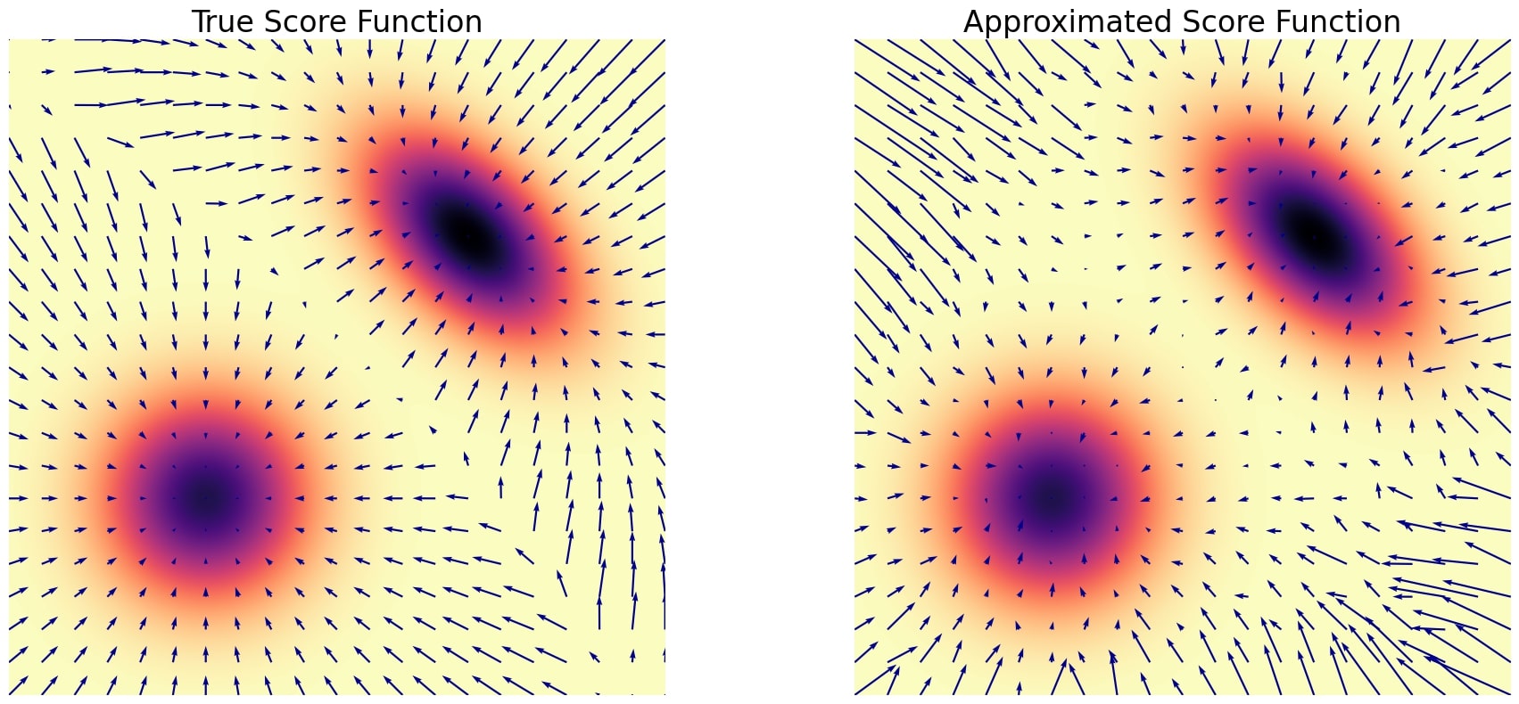
Figure 2. On the left the exact score of the Gaussian mixture, and on the right the approximated version using a 3-layer MLP trained with the Gaussian denoising loss (MSE). Note that the score is well approximated in high density regions, but is less precise in low density regions.

Additional results ³ show that the MSE training objective is actually equivalent to the score matching objective, which explicitely tries to match the score function with the output of the network.

$$\mathbb{E}_{x, y} \left[ \|D_\theta(y) - x\|^2 \right] \equiv \mathbb{E}_{y} \left[ \left\| \frac{D_\theta(y) - y}{\sigma^2} - \nabla_y \log p(y) \right\|^2 \right]$$

So training our neural nets to remove Gaussian noise is indeed equivalent to learning the underlying score function of our training data.

Related works

A whole lot of other methods have already tried to tackle the self-supervised denoising problem. In the paper, the authors focus their comparisons with two families of methods:

• Noise2X: the first family is about integrating additional degradation to images to create artificial pairs
• SURE: the second one is based on Stein’s Unbiased Risk Estimate, which doesn’t require pairs at all

Noise2X methods

The general idea is to take a noisy image $y$, and degrade it further to create $y'$. The noisy image $y$ then acts as a label, and the neural network will try to remove this additional degradation.

$$\mathcal{L}_{Noise2X} = \| y' - D_{\theta} (y)\|^2$$

There are a lot of papers that follow this framework.

For instance in Noise2Noise ⁴, $y'$ is simply produced by taking another noise realization of the same image $y$. Of course this is really hard to do in practice, but it still highlights that clean labels are not required.

Another example is Noise2Void ⁵ where $y'$ is produced by adding blind spots in $y$.

Stein’s Unbiased Risk Estimate (SURE)

Another completely different line of work is based on Stein’s Unbiased Risk Estimate ⁶ which has been adapted ⁷ to formulate a loss function without using clean labels.

$$\mathcal{L}_{SURE} = \| y - D_{\theta} (y)\|^2 + 2 \sigma^2 \mathrm{div} D_{\theta} (y)$$

Tweedie-like formulas

There are actually equivalents of the Tweedie formula for other noise distributions. Indeed Gaussian noise is cool but it is very simple. In medical imaging, most of the noise we encounter is not Gaussian but rather Poisson or Gamma. Here’s a visual reference of what these noises look like:

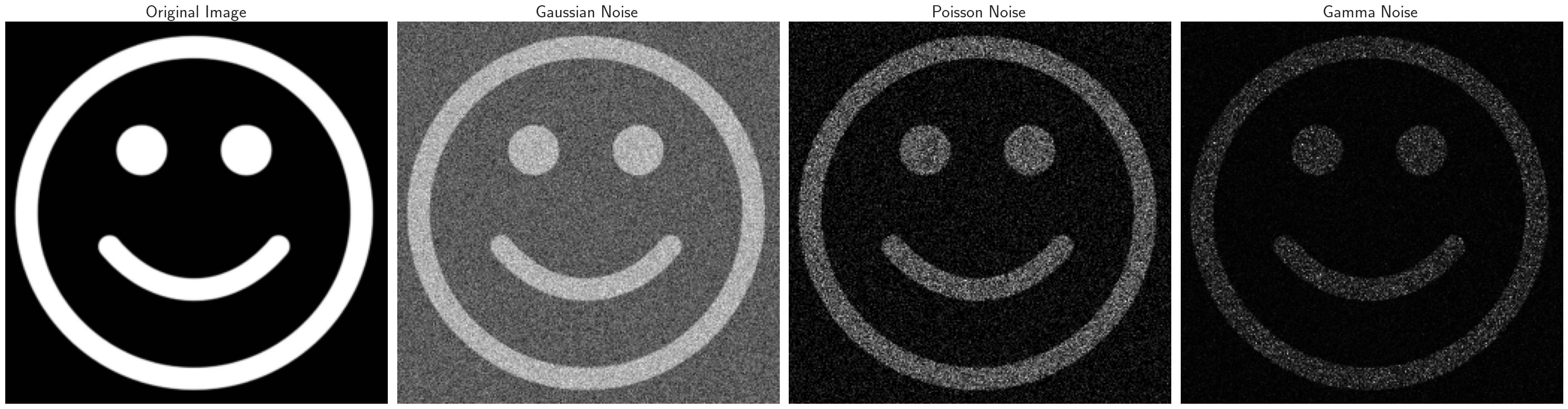
Figure 3. Exemple of corruptions with different noise distributions. Gaussian noise is additive, so it's uniform on the whole image. Poisson and Gamma are multiplicative, meaning they have no effect where there is no data. Gamma noise being more heavy-tailed than Poisson noise, it causes brighter spots on the image.

These expressions were in part derived in 2011 ² and rediscovered / extended in this paper. Here are the expressions for a few distributions of interest:

• Gaussian noise:

$$\mathbb{E} \left[ x \mid y \right] = y + \sigma^2 \nabla \log p(y)$$

where $\sigma$ is the variance of the noise.

• Poisson noise:

$$\mathbb{E} \left[ x \mid y \right] = \left( y + \frac{\zeta}{2} \right) \exp \left( \nabla \log p \left( \frac{y}{\zeta} \right)\right)$$

where $\zeta$ is an “artificial parameter” to control the strength of the Poisson noise.

• Gamma noise:

$$\mathbb{E} \left[ x \mid y \right] = \frac{\beta y}{(\alpha - 1) - y \nabla \log p(y)}$$

$\alpha$ and $\beta$ are the parameters of the Gamma distribution

Score estimation

It’s now clear that we can denoise images from any type of noise, as long as we have access to the score function of the perturbed distribution $\nabla \log p(y)$. Indeed we could just plug it in one of the formulas and get the denoised estimat $\mathbb{E} \left[ x \mid y \right]$. To do so the authors use denoising score matching ³, which means perturbing the already noisy images with a Gaussian noise.

$$\mathcal{L}_{DSM} = \| y - D_{\theta}(y + \sigma \epsilon) \|^2$$

where $\sigma$ is the variance of the Gaussian noise and $\epsilon \sim \mathcal{N}(0, 1)$.

To do this, they use a slightly modified version of a denoising autoencoder called an Amortized Residual DAE (AR-DAE). It takes the specific form:

$$D_{\theta} (x) = x + \sigma^2 R_{\theta} (x)$$

So basically just a skip connection and a ponderation depending on the noise level of the inputs.

The loss is then:

$$\mathcal{L}_{AR-DAE} = \| \epsilon + \sigma R_{\theta}(y + \sigma \epsilon) \|^2$$

where again $\sigma$ is the variance of the Gaussian noise and $\epsilon \sim \mathcal{N}(0, 1)$.

So the same strategy can be used (same network, same training), no matter the noise distribution. But you need to retrain for each noise distribution. You also need to know which type of noise is present in your data, and it also needs to be in the exponential family. For instance in emission tomography, the noise is known to be Poisson, but in ultrasound and magnetic resonance imaging, the noise distribution is harder to model. Another such instance of complex noise modelisation is the single-pixel camera.

Results

The authors simulate noisy observations by corrupting natural images with Gaussian, Poisson, or Gamma noise. Their method demonstrates strong performances, outperforming SURE and Noise2X, and approaching the results of fully supervised neural networks. In their experiments, the same network architecture is used across all training objectives, including the fully supervised setting where the model is trained with paired ground-truth and noisy images. As expected, the fully supervised setup yields the highest performance, which is confirmed empirically. However, as previously noted, acquiring clean ground-truth data for training is often difficult or infeasible in many real-world scenarios.

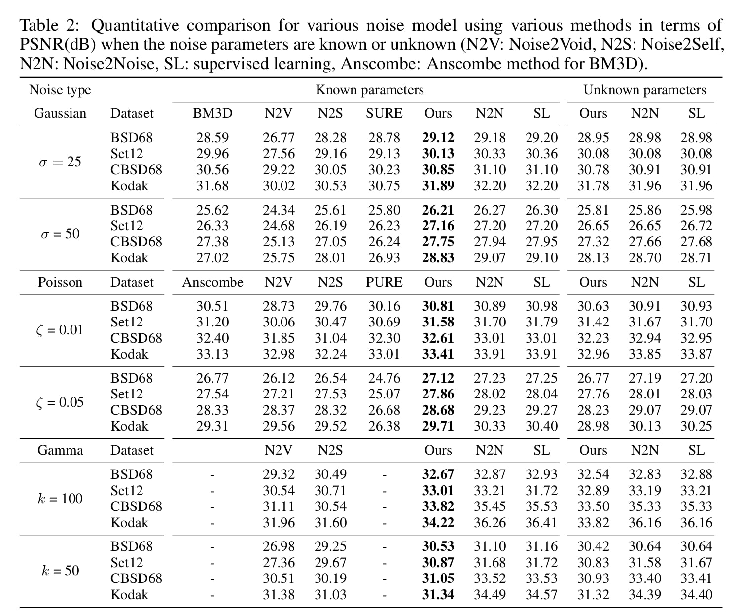
Figure 4. Results of their denoising experiments. Note how close they are to the fully supervised networks (SL column).

And in Figure 5 you can find some examples of denoised images.

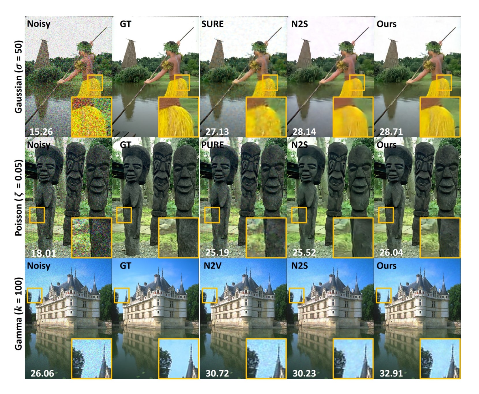
Figure 5. Denoising results on a few images.

References

1. Plug-and-Play Image Restoration With Deep Denoiser Prior, Kai Zhang et al., 2022 ↩

2. Tweedie’s Formula and Selection Bias, Bradley Efron et al., 2011 ↩ ↩²

3. A Connection Between Score Matching and Denoising Autoencoders, Pascal Vincent et al., 2011 ↩ ↩²

4. Noise2Noise: Learning image restoration without clean data, Alexander Krull et al., 2018 ↩

5. Noise2Void-learning denoising from single noisy images, Alexander Krull et al., 2019 ↩

6. Estimation of the mean of a multivariate normal distribution, Charles Stein, 1981 ↩

7. Training and Refining Deep Learning Based Denoisers without Ground Truth Data, Shakarim Soltanayev et al., 2018 ↩