Spiking Neural Networks
Introduction
Artificial neural networks are the cornerstone of modern artificial intelligence algorithms. However, despite their impressive performances, they still have their respective shortcoming, notably the enormous power required to train and run inference. This has motivated research into spiking neural networks.
Many reasons justify the interest in spiking neural networks, two of which are
- Biological plausibility
- Temporal and event-driven processing, which allows for sparse and energy-efficient computation.
The format for this review is based on the class GEI723 - Neurosciences computationnelles et applications en traitement de l’information at Sherbrooke University. The goal of this review will be to introduce the anatomical and physiological concepts of biological neurons before explaining how neurons can be modeled by a computer. Finally, a paper will be presented showing one of many ways a spiking neural network can be trained.
Anatomy and physiology
Neuron components
To appropriately model neurons in a computer, a certain number of concepts must be understood. This section will quickly introduce these concepts. A neuron, as depicted in the following figure, is composed of many parts such as
- Nucleus: Main part of the cell body.
- Dendrites: Part of the neuron that receives inputs from other neurons.
- Axon: Cable-like structure that carries the neuron signal.
- Axon terminal: End of the neuron from which connections to other neurons are made (through neurotransmitter)
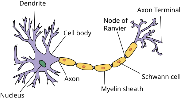
Figure 1. Illustration of a Neuron 1
Membrane potential
The neuron is separated from the outside of the cell by the neuron membrane. This separation causes a difference in electrical potential between the inside and outside. The change in this potential is what allows neurons to transmit signals, as will be explained later.
At rest, the membrane potential is around -70 mV.
The number of ions inside and outside the cell membrane defines the membrane potential. The main ions that affect the membrane potential are
- Potassium (\(K^+\)) : Positive ions, more prevalent inside the cell.
- Sodium (\(Na^+\)): Positive ions, more prevalent outside the cell.
- Calcium (\(Cl^-\)): Negative ions, more prevalent outside the cell.
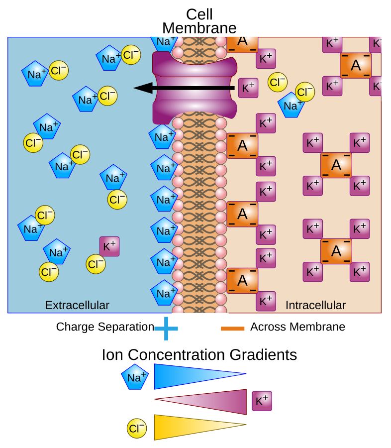
Figure 2. Illustration of a cell membrane 2
The membrane potential can be expressed mathematically with the Goldman-Hodgkin-Katz (GHK) equation,
\[v_m = \frac{RT}{F} ln \frac{P_K [ K^{+} ]_{out} + P_{Na} [ Na^{+} ]_{out} + P_{Cl} [ Cl^{-} ]_{out}}{P_K [ K^{+} ]_{int} + P_{Na} [ Na^{+} ]_{int} + P_{Cl} [ Cl^{-} ]_{int}}\]where
- \(P_{ion}\) is the permeability of the membrane for a given ion.
- \([ion]_{out}\) is the concentration of an ion outside the neuron
- \([ion]_{in}\) is the concentration of an ion inside the neuron.
Action potential
Due to an input stimulus, the membrane potential can change. This change in membrane potential affects the membrane’s permeability to different ions. If the input stimulus is large enough causing the membrane potential to surpass the threshold (-55 mV) an action potential (spike) is generated.
The increase in membrane voltage causes the permeability of sodium ions to increase leading to sodium ions rushing into the cell further increasing the membrane potential. At the peak of the action potential, the sodium permeability goes back down and the potassium permeability increases causing an outflux of potassium ions causing the membrane potential to fall, below the resting potential.
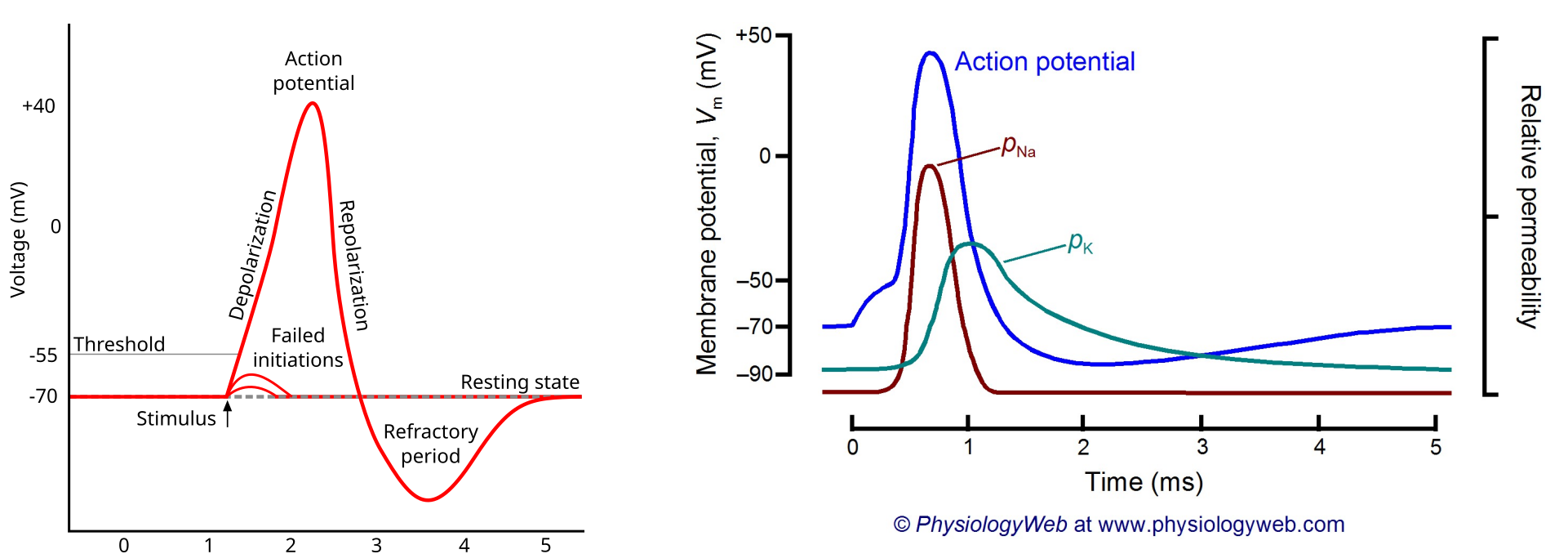
Figure 3. (left) Membrane potential during action potential 3. (right) Membrane permeability during action potential 4.
The action potential is followed by a refractory period. Two types of refractory periods exist:
- The absolute refractory period during which the neuron physically cannot fire.
- The relative refractory period during which the neuron can fire given a large enough stimulus.
Synapses
Synapses connect neurons. When a synapse connects two neurons we refer to the first neuron as the pre-synaptic neuron and the second neuron as the post-synaptic neuron. Synapse can be either excitatory or inhibitory causing an increase or decrease the post-synatic neuron activity.
There are two main types of synapses: chemical and electric.
- Chemical: Electrical activity in the pre-synaptic releases neurotransmitters that can either excite or inhibit the post-synaptic neuron.
- Electric: Special channels between pre- and post-synaptic neurons allow the changes in voltage of the pre-synaptic neuron to induce a change in the post-synaptic neuron.
Learning
It is mostly considered that learning in the brain occurs when a synapse is modified due to pre-synaptic stimulation of post-synaptic cells. This process is known as Hebbian learning. Spike-timing-dependent plasticity (STDP) is the process that adjusts the weights of synapses according to the timing of pre-synaptic and post-synaptic spikes.
Different paradigms of STDP exist but the most common is the following:
- Synaptic weights increase when the pre-synaptic spike induces a post-synaptic spike.
- Synaptic weights decrease when the post-synaptic neuron spikes before the pre-synaptic neuron.
The size of the weight change is dependent on the time between the two spikes.
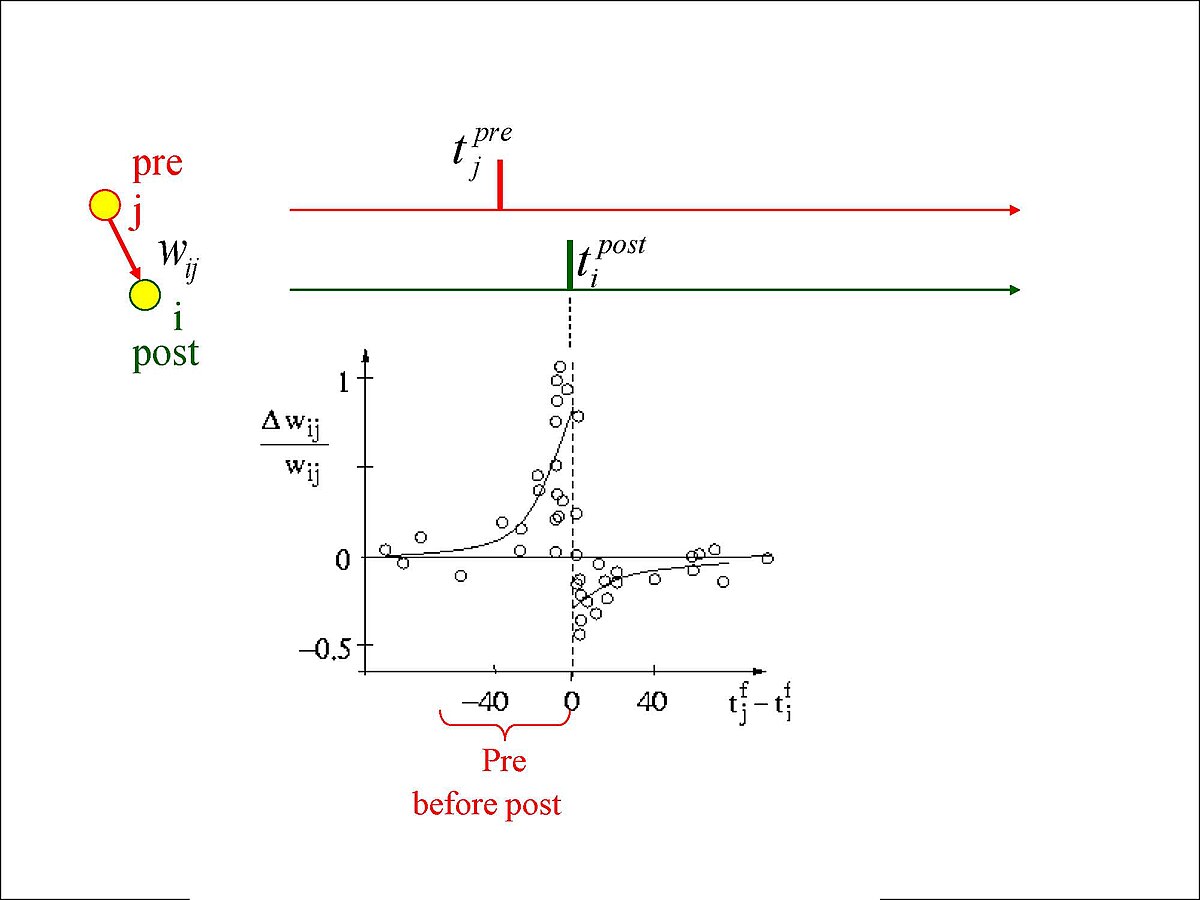
Figure 4. Example of STDP 5.
Modeling Spiking Neural networks
Neuron models
Many mathematical models have been proposed to represent the behavior of a neuron. Often, these models have to balance biological plausibility and computational complexity.
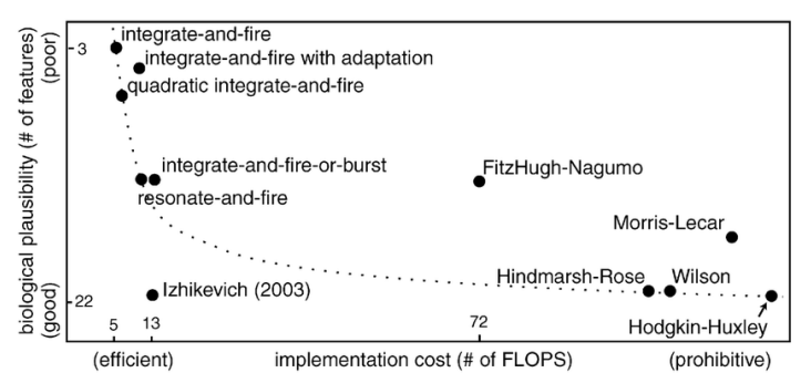
Figure 5. Neuron models and their relative complexities 6.
The most realistic, but also most complex, model is the Hodgkin–Huxley. The model is made of several differential equations representing the neuron potential according to inputs.
The simplest way to model a neuron is with the integrate and fire (IF). This neuron accumulates voltage from its input and when the voltage reaches a threshold it fires a spike. The voltage is reset to the resting voltage and the neuron cannot fire during a refractory period. A leaky version known as the leaky integrate and fire (LIF) loses voltage according to a differential equation.
Input encoding
To interact with mathematical models of neurons, we must transmit data to them. To do so, we must encode the data in a way the neurons can receive it. This is done by input neurons which spike according to different encoding schemes. The two most popular schemes are time to spike and rate coding.
- Time to spike coding: The neuron spikes once with a delay determined by the input amplitude.
- Rate code: the neuron spikes at a frequency determined by the input amplitude (with optional stochasticity)
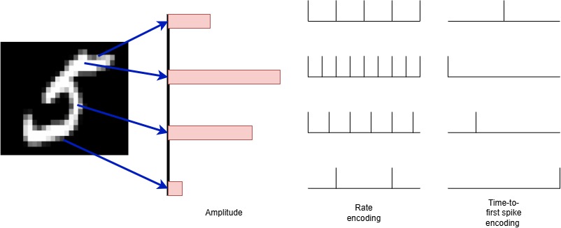
Figure 6. Example of input encodings.
Example of neuron function and interaction:
Different Python packages can be used to implement neuron models. The packages allow the modeling of neurons using differential equations and solve these questions for simulations.
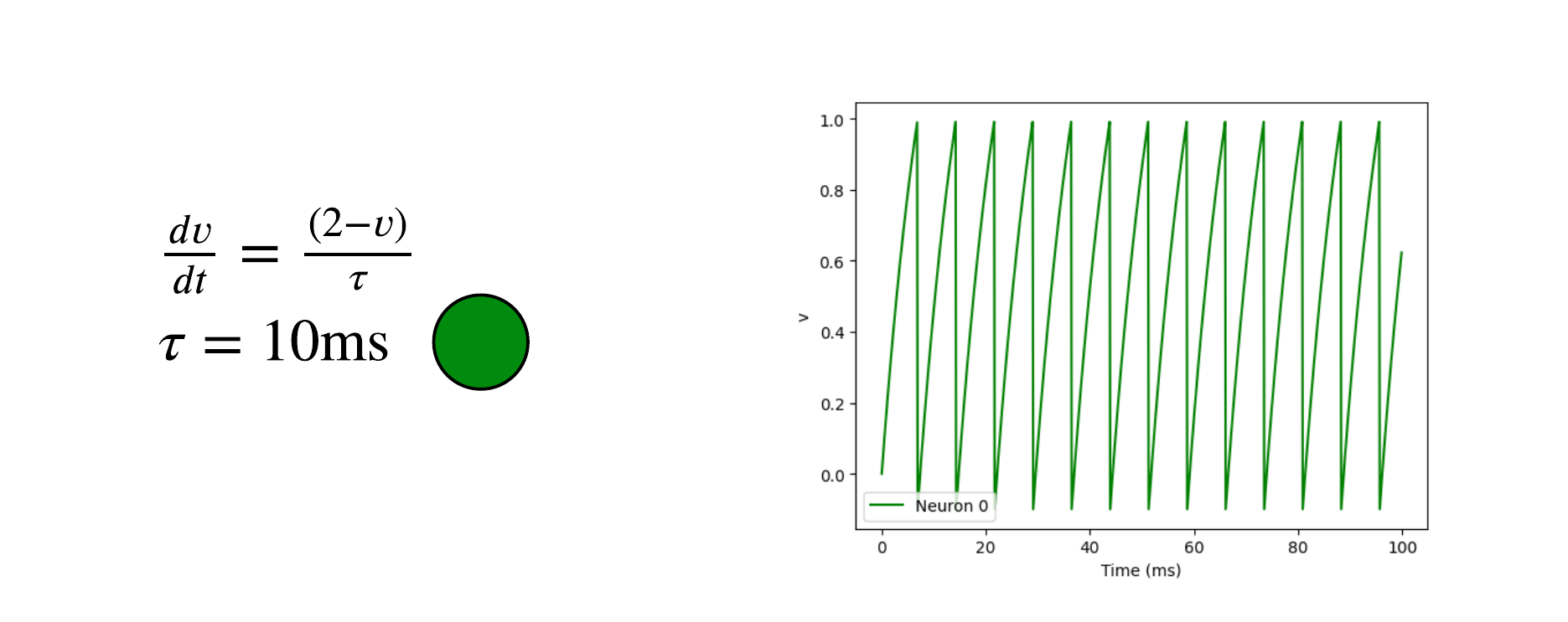
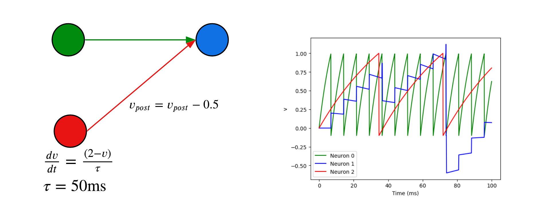
Here are examples of neuron models using the Python package Brain2 7. All neurons have a threshold of 1V and a reset voltage of -0.5V.
The first neuron is a leaky integrate and fire. Due to its differential equations, the voltage increases and fires on its own.
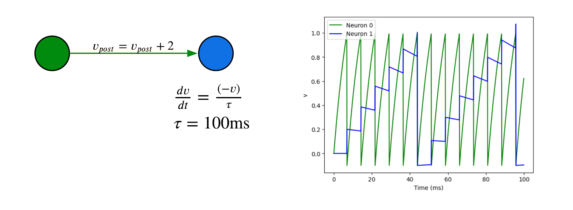
We can add a second neuron with a synapse. When the pre-synaptic neuron (green) spikes, the voltage of the post-synaptic neuron increases by 0.2V.
We can add a second neuron with a synapse. Here the red pre-synaptic neuron is connected to the blue neuron with an inhibitory synapse and reduces its voltage by 0.5V when it spikes.
import numpy as np
from brian2 import *
import matplotlib.pyplot as plt

# Define the equation for the neuron (LIF)
eqs = '''
    dv/dt = (I-v)/tau : 1
    I : 1
    tau : second
'''
# Define the neurons.
G = NeuronGroup(3, eqs, threshold='v>1', reset='v = -0.1', method='euler')
G.I = [2, 0, 2]
G.tau = [10, 100, 50]*ms

# Comment these two lines out to see what happens without Synapses
S = Synapses(G, G, on_pre='v_post += 0.2')
S.connect(i=0, j=1)

# Comment these three lines to remove the inhibitor synapse.
S2 = Synapses(G, G, on_pre='v_post -= 0.5')
S2.connect(i=2, j=1)
S2.delay = '2*ms'

M = StateMonitor(G, 'v', record=True)

run(100*ms) # Run the simulation for 100 ms.

plot(M.t/ms, M.v[0], label='Neuron 0')
plot(M.t/ms, M.v[1], label='Neuron 1')
plot(M.t/ms, M.v[2], label='Neuron 2')
xlabel('Time (ms)')
ylabel('v')
legend();
Learning with Spiking Neural Networks - Article Review
To better understand how all this can be applied, the rest of this review will be dedicated to the review of a paper. While spiking neural networks can be used in many ways, this paper proposes a simple method for training a spiking neural network.
Diehl, P., & Cook, M. (2015). Unsupervised learning of digit recognition using spike-timing-dependent plasticity. Frontiers in Computational Neuroscience, 9.
The paper is not on Arxiv, please refer to the paper for the original figures.
Introduction
In this paper, the authors propose a method to do unsupervised MNIST classification with a spiking neural network training with STDP.
The paper contains many details important for implementation but less for understanding the general idea. Many of these details will be omitted.
Method
Neuron model
All neurons are modeled using the leaky integrate and fire model. In this case, the neuron potential is given by
\[\tau \frac{dV}{dt} = (E_{rest} - V) + g_e(E_{exc} - V) + g_i(E_{inh}- V)\]where
- \(E_{rest}\) is the resting membrane potential.
- \(E_{exc}\) and \(E_{inh}\) are the equilibrium potentials of excitatory and inhibitory synapses.
- \(g_e\) and \(g_i\) are the conductances of excitatory and inhibitory synapses.
- \(\tau\) is a time constant
Each neuron has a threshold potential \(v_{thresh}\) at which the neuron spikes and a reset potential \(v_{reset}\) after the spike.
The authors explain that they use biologically plausible ranges for almost all the parameters. They do not give these values in the code but direct readers to the code. Unfortunately this means that some values are not explained. For example \(E_{exc}\) seems to be 0 according to the code without any explanation.
Synapse model
Instead of directly modifying the potential of a cell, the synapse affects the conductance. Each synapse has a weight \(w\) which is used to increase the post-synaptic neuron’s conductance. If the synapse is excitatory, the excitatory conductance \(g_e\) of the post-synaptic neuron is increased by \(w\) when the pre-synaptic neuron fires. The same applies to the inhibitory synapse.
Both the excitatory and inhibitory conductances decay using the following equation \(\tau_{g} \frac{dg}{dt} = - g\)
where \(\tau_{g}\) is a time constant for the conductance (different for excitatory and inhibitory).
Network architecture
The network consists of 3 neuron layers
- The input layer contains 784 (28 x 28) neurons, one for each pixel in the input image. These neurons encode the pixel values into spikes using a frequency encoding.
- The second layer contains N excitatory neurons.
- The third layer contains N inhibitory neurons.
The synapses in the neuron are shown in the following figure (network with 3 input neurons and 4 excitatory/inhibitory neurons).
- All input neurons are connected to each excitatory neuron.
- The excitatory neurons are connected to the inhibitory in a one-to-one fashion.
- The inhibitory neurons are connected to all excitatory except the one with which it already has a connection.
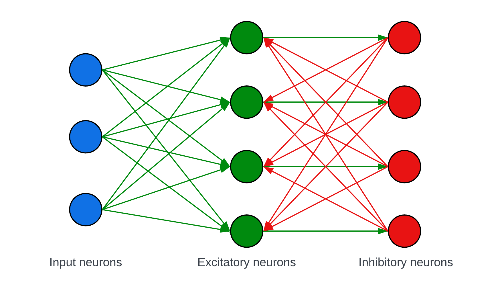
Figure 7. Network architecture
Connection all the excitatory neurons to inhibitory neurons will allow the first neuron to spike to suppress all the other excitatory neurons. This concept is called lateral inhibition.
Learning
The network only learns the input synapse using STDP. The weights between the excitatory and inhibitory neurons are fixed in both directions.
This section is poorly explained in the paper and requires an understanding of many other references. However, the general concepts of STDP are used. If an input neuron spikes before an excitatory neuron, their synaptic weight is increased. If the excitatory spikes before the input neuron, the synaptic weight is decreased.
Input encoding
Each of the 784 input neurons is fed a Poisson-distributed spike train. The rate of the spike train is proportional to the pixel intensity of input images. The firing rates are between 0 and 63.75 Hz (which corresponds to the maximum pixel value, 255, divided by 4).
Training
During training, images are presented to the network one by one. Each input is presented for 350 ms. If there are less than 5 spikes in this period in the excitatory neuron layer, the image is presented for an additional 350 ms with a firing rate increased by 32 Hz. After each image, there is a 150 ms waiting phase to allow the neuron variables to reset.
The concept of training can be hard to understand but can be explained as follows: Each synapse weight is initialized randomly. As the first image is shown, some of the excitatory neurons will fire due to the input stimulus. These excitatory neurons will trigger their corresponding inhibitory neurons and will trigger lateral inhibition. As the input neurons caused some of the excitatory to fire, the corresponding synaptic weights will be increased by the process of STDP. When another image is presented, other neurons will likely be excited and the same process will occur.
Homeostasis
It is important that all neurons have approximately the same firing rate. This prevents one neuron from dominating the others. To ensure a controlled firing rate, homeostasis is implemented as an adaptive threshold. The threshold for each neuron is given by the following equation:
\[v_t = v_{thresh} + \theta\]The value of \(theta\) increases each time the neuron fires and decreases exponentially. The threshold is therefore higher if several discharges occur in succession and decreases again if the discharges are spaced apart.
Inference
Once training is complete, the synaptic weights and the adaptive thresholds are fixed. The images of the training set are once again passed through the network. Each excitatory neuron is assigned a class corresponding to the image that caused the most activity (i.e. the most spikes).
During inference, a new image is presented and the predicted class is given by the group of neurons with the highest average firing rate.
Results
The authors implement various versions of their model, testing the effect of the number of excitatory neurons, different STDP rules, and comparing to other spiking neural network architectures. Details are not important to understanding the methodology. The best version of their method achieves an accuracy of 95% on the MNIST test set.
During training (and once it is complete), the weights of classification neurons for each class can be viewed in 28x28 pixel images showing their receptive field. The final image was generated by training on a limited number of epochs with only 1000 training images. Training with the full dataset for a longer period would result in clearer numbers (see paper figures).
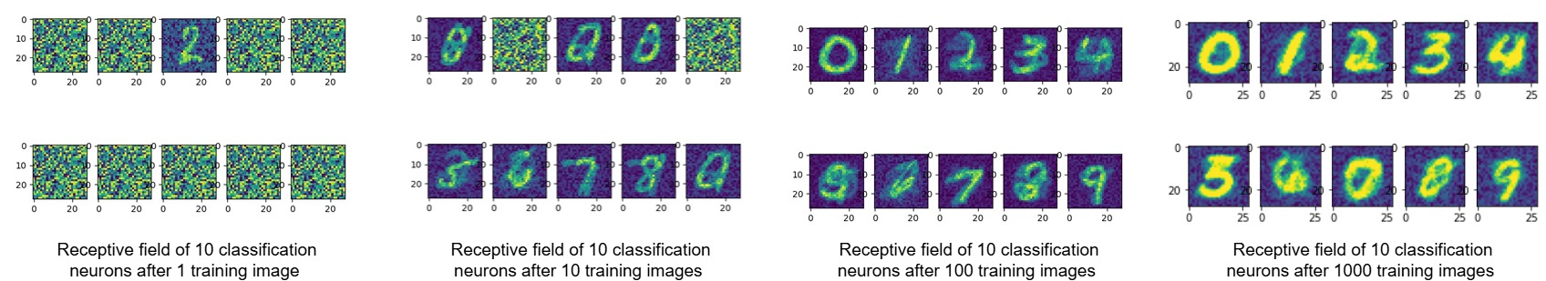
Figure 8. Receptive fields of classification neurons during training.
Code
The authors release their code https://github.com/peter-u-diehl/stdp-mnist.
A simpler version is provided in this Google Colab. Some equations are different from the default settings explained in this review.
What to remember from this review.
- Biological neurons (modeled by differential equations) work on spikes, not continuous inputs.
- Spiking neural networks can be trained with STDP. Contrary to backpropagation which carries global information, STDP is only applied locally.
- Spiking neural networks have the potential to greatly reduce the computational cost of neural networks. But why ?
Imagine a single artificial neuron (dot product) and a spiking neuron both receiving the following input: \(x = [0, 0.1, 0.01, 0.02, 5, 100, 0.4]\). The artificial neuron will compute the dot product with a weight vector \(w\). Even if many of the inputs will have little effect on the output, the computation is still required. The spiking neuron, on the other hand, assuming it is preceded by other spiking neurons, will only compute the inputs for which a spike is generated. This means that small values in the input \(x\) that do not generate a spike are not computed.
Therefore, spiking neural networks offer a sparse alternative to the dense computation of traditional artificial neural networks.
References
-
https://commons.wikimedia.org/wiki/File:Neuron.svg ↩
-
https://commons.wikimedia.org/wiki/File:Basis_of_Membrane_Potential2-en.svg ↩
-
https://commons.wikimedia.org/wiki/File:Action_potential.svg ↩
-
https://www.physiologyweb.com/lecture_notes/neuronal_action_potential/figs/neuronal_action_potential_timecourse_of_pna_and_pk_jpg_zgn9dUl70MnJPf2CqaZ5uoL3BBD6r9fW.html ↩
-
https://commons.wikimedia.org/wiki/File:STDP-Fig1.jpg ↩
-
https://www.izhikevich.org/publications/whichmod.pdf ↩
-
https://brian2.readthedocs.io/en/stable/ ↩