Delving into Deep Imbalanced Regression
Highlights
- Defines Deep Imbalanced Regression (DIR) as learning from imbalanced data with continuous targets.
- Introduces two distribution smoothing methods: Label Distribution Smoothing (LDS) and Feature Distribution Smoothing (FDS).
- Benchmarks performance on several real-world datasets.
- Code available on GitHub.
Related Work
Regression tasks are defined the estimation of continuous targets (e.g age prediction, depth estimation) whereas classification tasks are defined by the prediction of a categorical label (e.g. cat or dog). In real-world datasets, both regression and classification tasks face imbalanced datasets, which make non-adapted training performance drop.
Imbalanced Classification
Many prior works have focused on imbalanced classification problems. Two main approaches emerged:
- Data-based methods: under-sampling majority classes or over-sampling minority classes (e.g., SMOTE 1 2 3).
- Model-based methods: modifying loss functions via re-weighting to compensate for imbalance 4 5.
Recent studies also show that semi-supervised and self-supervised learning can improve performance under imbalance 6. While these methods can partially transfer to regression, they have intrinsic limitations due to the continuous nature of regression targets.
Imbalanced Regression
Imbalanced regression has been less explored. Most existing studies adapt SMOTE to regression by generating synthetic samples via input-target interpolation or Gaussian noise augmentation 7. However, these methods, inspired by classification strategies, fail to leverage the continuity in the label space. Moreover, linear interpolation may not produce meaningful synthetic samples.
The proposed methods in this paper differ fundamentally and can complement these prior approaches.
Methods: Label and Features Distribution Smoothing (LDS & FDS)
Problem Setting
Let \(\{ (x_i, y_i) \}_{i=1}^N\) be the training set, where \(x_i \in \mathbb{R}^d\) is the input, where d in the dimension of the input, \(y_i \in \mathbb{R}\) is the continous target and \(N\) the number of samples. We can divide the label space \(\mathcal{Y}\) into \(B\) bins with equal intervals: \([y_0, y_1[, [y_1, y_2[, .., [y_{B-1}, y_B[\). The defined bins reflect a minimum resolution we care for grouping data in a regression task (ex: in age estimation, \(\delta y = y_{b+1} - y_b = 1\) year). Finally, we denote \(z = f(x; \theta)\) the feature for x, where \(f(x; \theta)\), is parameterized by a deep neural network model with parameter \(\theta\). The final prediction \(\hat{y}\) is given by a regression function \(g(z)\).
Label Distribution Smoothing (LDS)
Motivation Example
To motivate LDS, the authors compare categorical labels (CIFAR-100) with continuous labels (IMDB-WIKI). Both datasets are subsampled to simulate imbalance, as illustrated on top of Firgure (1).
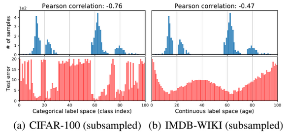
Figure 1.Comparison on the test error distribution (bottom) using same training label distribution (top) on two different datasets: (a) CIFAR-100, a classification task with categorical label space. (b) IMDB-WIKI, a regression task with continuous label space.
ResNet-50 trained on CIFAR-100 yields a test error distribution strongly correlated with label density (high negative Pearson correlation). For IMDB-WIKI, the test error distribution is smoother and less correlated with label density (Pearson = -0.47).
This example shows that, given the continuous caracteristic of labels, the network can learn from the neighborhood and give good performance on interpolation. So the imbalance seen by the network is different from the empirical class imbalance. Hence, compensating for data imbalance based on empirical label density is inaccurate for the continuous label space.
LDS Formulation
Label Distribution Smoothing (LDS) applies kernel density estimation to smooth the empirical label distribution:
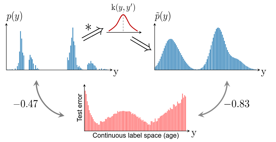
Figure 2.Label distribution smoothing (LDS) convolves a symmetric kernel with the empirical label density to estimate the effective label density distribution that accounts for the continuity of labels
A symmetric kernel is any kernel that satisfies: \(k(y, y') = k(y', y) \quad\) and \(\quad \nabla_y k(y, y') + \nabla_{y'} k(y', y) = 0, \quad \forall y, y' \in \mathcal{Y}.\) (e.g., Gaussian or Laplace). The symmetric kernel characterizes the similarity between target values \(y'\) and any \(y\) w.r.t. their distance in the target space. Thus, LDS computes the effective label density distribution as:
\[\tilde{p}(y') = \int_{\mathcal{Y}} k(y, y') p(y) \, dy\]where \(p(y)\) is the number of appearances of label of \(y\) in the training data, and \(\tilde{p}(y')\) is the effective density of label \(y'\).
The smoothed distribution correlates better with error distributions (Pearson = -0.83). Standard imbalance mitigation methods (e.g., re-weighting) can then be applied using \(\tilde{p}(y')\).
Feature Distribution Smoothing (FDS)
The authors followed the intuition that continuity in the target space should create a corresponding continuity in the feature space. That is, if the model works properly and the data is balanced, one expects the feature statistics corresponding to nearby targets to be close to each other.
Motivation example
The authors trained a plain model on the images in the IMDB-WIKI dataset to infer a person’s age from visual appearance. They focused on the feature space, i.e. z, grouped them within the same target age value and computed feature statistics (i.e. mean and variance) with respect of each bin, denoted \(\{\mu_b, \sigma_b\}\). To visualize the similarity between feature statistics, the authors select an anchor bin \(b_0\), and calculate the cosine similarity of the feature statistics between \(b_0\) and all other bins.
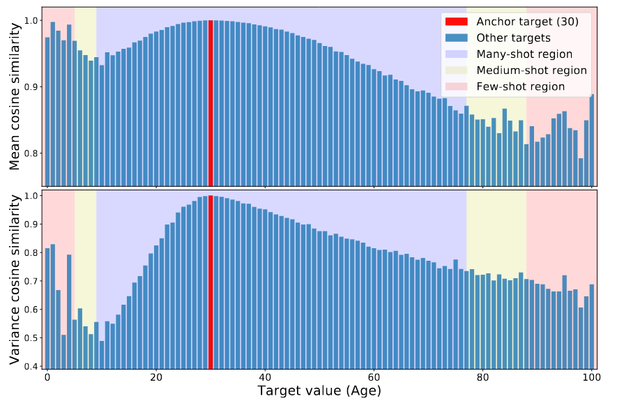
Figure 3. Feature statistics similarity for age 30. Top: Cosine similarity of the feature mean at a particular age w.r.t. its value at the anchor age. Bottom: Cosine similarity of the feature variance at a particular age w.r.t. its value at the anchor age. The color of the background refers to the data density in a particular target range.
The figure above shows that the feature statistics around the anchor b0 = 30 are highly similar to their values at b0 = 30. So, the figure confirms the intuition that when there is enough data, and for continuous targets, the feature statistics are similar to nearby bins. Interestingly, the figure also shows a high similarity between the age 0 to 6, that have a very few samples, with b0=30. This unjustified similarity is due to data imbalance. Specifically, since there are not enough images for ages 0 to 6, this range thus inherits its priors from the range with the maximum amount of data, which is the range around age 30.
FDS Formulation
FDS aims at transfering the feature statistics between nearby target bin, so that it calibrates the potentially biased estimates of feature distribution, especially for underrepresented target values, with the following procedure:
- Compute feature mean \(\mu_b\) and covariance \(\Sigma_b\) per bin:
- Smooth the feature statistics using kernel \(k(y_b, y_{b'})\):
- Re-calibrate the feature:
The FDS algorithm can be integrated to the network with a feature calibration layer after the final feature map. During the training, its employs a momentum update (exponential moving average) of the running statistics \(\{\mu_b, \Sigma_b\}\) across each epoch. Correspondingly, the smoothed statistics \(\{\tilde{\mu}_b, \tilde{\Sigma}_b\}\) are updated across different epochs but fixed within each training epoch.
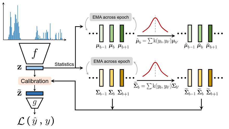
Figure 3. Feature distribution smoothing (FDS) introduces a feature calibration layer that uses kernel smoothing to smooth the distributions of feature mean and covariance over the target space.
FDS can be integrated with any neural network model, as well as any past work on improving label imbalance.
Results
Benchmark DIR
Datasets
Age Prediction. IMDB-WIKI-DIR & AgeDB-DIR: Imbalanced training set, manually constructed balanced validation & test set
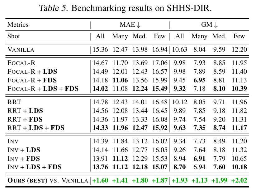
Health Condition Score. SHHS-DIR, based on the SHHS dataset, containing night EEG, ECG as inputs and a general health score is the output.
Baselines
-
Vanilla Model: a model that does not include any technique for dealing with imbalanced data.To combine the vanilla model with LDS, the authors re-weighted the loss function by multiplying it by the inverse of the LDS estimated density for each target bin
-
Synthetic Samples: Using SMOTER and SMOGN as baselines 1 2. SMOTER first defines frequent and rare regions using the original label density, and creates synthetic samples for rare regions by linearly interpolating both inputs and targets. SMOGN further adds Gaussian noise to SMOTER. LDS can be directly used for a better estimation of label density when dividing the target space.
-
Error Aware Loss: Inspired from the Focal Loss 8, the authors introduce Focal-R Loss = \(\frac{1}{n} \sum_{i=1}^{n} \sigma(\lvert \beta e_i \rvert) ^{\gamma} e_i\), where \(e_i\) is the L1 error for the i-th sample, \(σ(·)\) is the sigmoid function, and \(\beta, \gamma\) are hyper-parameters. To combine Focal-R with LDS, the authors multiply the loss with the inverse frequency of the estimated label density.
-
Two-stage training: the authors propose a regression version called regressor re-training (RRT), where in the first stage the authors train the encoder normally, and in the second stage freeze the encoder and re-train the regressor g(·) with inverse re-weighting. When adding LDS, the re-weighting in the second stage is based on the label density estimated through LDS.
-
Cost-sensitive re-weighting: Since the authors divided the target space into finite bins, classic re-weighting methods can be directly plugged in. The authors adopt two re-weighting schemes based on the label distribution: inverse-frequency weighting (INV) and its square-root weighting variant (SQINV). When combining with LDS, instead of using the original label density, the authors use the LDS estimated target density.
Benchmarks
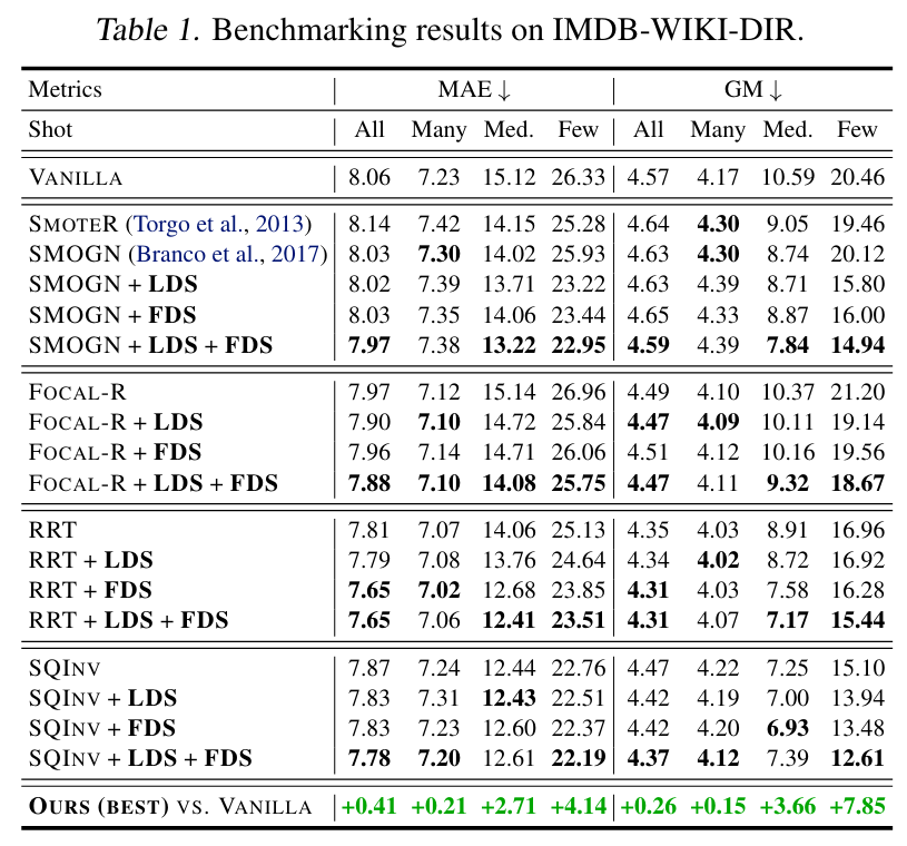
SMOTER and SMOGN can actually degrade the performance in comparison to the vanilla model. Moreover, within each group, adding either LDS, FDS, or both leads to performance gains, while LDS + FDS often achieves the best results. Finally, when compared to the vanilla model, using LDS and FDS maintains or slightly improves the performance overall and on the many-shot regions, while substantially boosting the performance for the medium-shot and few-shot regions.
Further Analysis
Interpolation & Extrapolation
To simulate a scenario of certain target values with no samples, the authors curated the age dataset on the training set, as shown on the figure below.
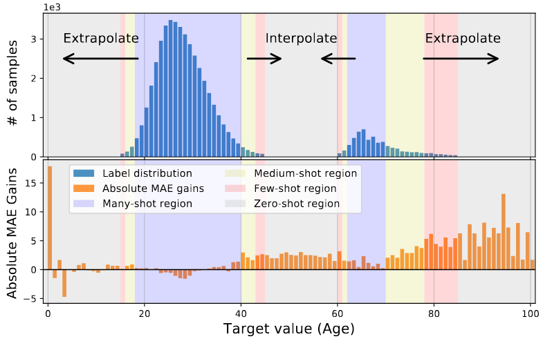
Figure 4. The absolute MAE gains of LDS + FDS over the vanilla model, on a curated subset of IMDB-WIKI-DIR with certain target values having no training data. The authors establish notable performance gains w.r.t. all regions, especially for extrapolation & interpolation
Understanding FDS
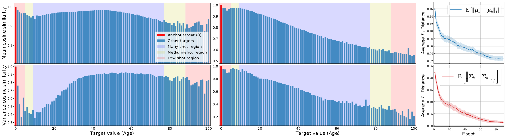
Figure 5. (a) Feature statistics similarity for age 0, without FDS (b) Feature statistics similarity for age 0, with FDS (c) L1 distance between the running statistics \( \{\mu_b, \Sigma_b\} \) and the smoothed statistics \(\{\tilde{\mu}_b, \tilde{\Sigma}_b\}\) during training.
As the figure indicates, since age 0 lies in a few-shot region, the feature statistics can have a large bias, i.e., age 0 shares large similarity with region 40 ∼ 80 as in Fig. 8(a). In contrast, when FDS is added, the statistics are better calibrated, resulting in a higher similarity only in its neighborhood, and a gradually decreasing similarity score as target value becomes larger. The L1 distance between the running statistics \(\{\mu_b, \Sigma_b\}\) and the smoothed statistics \(\{\tilde{\mu}_b, \tilde{\Sigma}_b\}\) during training is plotted in Fig. 8(c). Interestingly, the average L1 distance becomes smaller and gradually decreases as the training evolves, indicating that the model learns to generate features that are more accurate even without smoothing, and finally the smoothing module can be removed during inference.
Conclusion
The authors introduce the DIR task that learns from natural imbalanced data with continuous targets, and generalizes to the entire target range. The authors propose two simple and effective algorithms for DIR that exploit the similarity between nearby targets in both label and feature spaces.
References
-
Chawla, N. V., Bowyer, K. W., Hall, L. O., and Kegelmeyer, W. P. Smote: synthetic minority over-sampling technique. Journal of artificial intelligence research, 16:321–357 2002. ↩ ↩2
-
Branco, P., Torgo, L., and Ribeiro, R. P. Smogn: a preprocessing approach for imbalanced regression. In First international workshop on learning with imbalanced domains: Theory and applications, pp. 36–50. PMLR, 2017. ↩ ↩2
-
Branco, P., Torgo, L., and Ribeiro, R. P. Rebagg: Resampled bagging for imbalanced regression. In Second International Workshop on Learning with Imbalanced Domains: Theory and Applications, pp. 67–81. PMLR, 2018. ↩
-
Cao, K., Wei, C., Gaidon, A., Arechiga, N., and Ma, T. Learning imbalanced datasets with label-distribution-aware margin loss. In NeurIPS, 2019 ↩
-
Cui, Y., Jia, M., Lin, T.-Y., Song, Y., and Belongie, S. Class-balanced loss based on effective number of samples. In CVPR, 2019. ↩
-
Yang, Y. and Xu, Z. Rethinking the value of labels for improving class-imbalanced learning. In NeurIPS, 2020. ↩
-
Torgo, L., Ribeiro, R. P., Pfahringer, B., and Branco, P. Smote for regression. In Portuguese conference on artificial intelligence, pp. 378–389. Springer, 2013 ↩
-
Lin, T.-Y., Goyal, P., Girshick, R., He, K., and Doll ´ar, P. Focal loss for dense object detection. In ICCV, pp. 2980–2988, 2017. ↩