Metric Flow Matching for Smooth Interpolations on the Data Manifold

Highlights

• Modern generative models rely on constructing conditional paths between two distributions, but rely on the assumption of Euclidean geometry
• The authors introduces Metric Flow Matching (MFM), a simulation-free approach to force the vector field to stay close to the training data manifold.
• The code associated with the paper is available on the official GitHub repository.

 

Reminder on flow matching

This part is not intended an extensive guide on flow matching, only a quick introduction on the general concepts. For in depth explanations, see this blog post and this tutorial presented at NeurIPS 2024.

Let’s consider a source distribution \(p_0\) and a target distribution \(p_1\). We are looking to find a map \(f\) that pushes forward \(p_0\) to \(p_1\). More specifically,Flow Matching, in line with (continuous) Normalizing Flow and Diffusion Models, suppose that there exist a vector field \(u_t\) that can generate the distribution \(p_1\) starting at \(p_0\).

However, \(u_t\) is typically intractable and we need a workaround to estimate it. Without going into technical details, we model the vector field by a neural network \(v_{t,\theta}\), which is trained to minimize the following objective:

\[\mathcal{L}(\theta) = \mathbb{E}_{t, (x_0,x_1) \sim q} \lVert v_{t, \theta} (x_t) - \dot{x_t} \rVert ^2 = \mathbb{E}_{t, (x_0,x_1) \sim q} \lVert v_{t, \theta} (x_t) - (x_1 - x_0) \rVert ^2\]

where \(x_t\) are called the interpolants from \(x_0\) to \(x_1\). In practice, we use linear interpolants because we can compute their derivatives. If \(x_0\) and \(x_1\) are respectively drawn from \(p_0\) and \(p_1\), we compute their linear interpolation \(x_t = t x_1 + (1-t)x_0\), pass it through the neural network and try to match its output with the vector \(u_t = x_1 - x_0\).

Compared to related generative models, Flow Matching has several advantages:

• It provides a solution to Conditional Normalizing Flows, which previously needed simulation for generating vector fields, with heavy computational cost, making it unscalable to large datasets and inputs.
• The objective is simpler than DDPM and allows to find straighter paths for generation. Moreover, because of those straighter paths and the fact that the target vectors \(u_t\) are constant over time \(t\), it allows easier accelerating sampling techniques.
• Finally, contrary to standard diffusion models, the formalism of Flow Matching is not bounded by a Gaussian target distribution and thus allows to find generative paths between any source and target distributions.

 

Motivation

In many applications, such as image processing, the manifold hypothesis is reasonable assumption on the data distribution. It says that the data arises from a low-dimensional manifold \(\mathcal{M} \in \mathbb{R}^d\). In that case, the linear interpolants may not fall on the data manifold, which can be unwanted for some applications (Figure 1). The goal of the paper is to provide a scalable approach to tackle this issue.

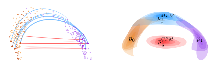
Figure 1. Source and target distributions in orange and purple. With straight interpolants, the densities reconstructed at time t=0.5 lies out of the data manifold.

 

Metric Flow Matching

The goal here is not to go into the mathematical details and proofs supporting the work. Feel free to dive into paper for more in-depth explanations.

Let’s informally introduce the concept of Riemannian manifold as follows. A Riemannian manifold is a smooth manifold, in the sense that it is locally Euclidean. There exists a map \(g\) assigning each point \(x\) of the manifold to an inner product \(\langle \cdot , \cdot \rangle\) defined on the tangent space of \(x\). We can represent this mapping by \(G(x)\) where \(G\) is a semi-definite positive matrix representing \(g\) in coordinates. We call geodesic a curve \(\gamma_t^*\) that connects two points of the manifold by minimizing the distance with respect to the local inner products, i.e.: \(\gamma_t^* = \underset{\gamma_t, \gamma_0=x_0, \gamma_1=x_1}{\arg \min} \int_{0}^{1} \lVert \dot{\gamma_t}_{g(\gamma_t)} \rVert dt\)

where \(\dot{\gamma_t}\) is the velocity. Geodesics tends to pass through regions where \(\lVert G(x) \rVert\) is small. They correspond to straight lines at constant speed in Euclidean geometry.

Metric Flow Matching is made of three main steps:

• Metric learning: the goal is to construct a metric that depends on the (empirical) data and that allows for the geodesics to stay close to the data manifold.
• Trajectories correction : in a second step, a neural network is trained to correct the linear interpolants and predict new interpolants that stay on the data manifold.
• Metric Flow Matching : finally, the nonlinear correction is used to train a second neural network that performs flow matching but can follow the trajectories learnt by the first network.

Metric learning

The authors discuss two metrics, LAND and RBF, but we will focus solely on the latter, as it is the one that can be used in higher dimensional problems.

They define a metric of the form \(G_{\text{RBF}} = (\text{diag}(\tilde{h}(x)) + \epsilon I)^{-1}\) with :

\[h_{\alpha}(x) = \sum_{k=1}^{K} \omega_{\alpha,k}(x) \exp{( - \frac{\lambda_{\alpha,k}}{2} \lVert x - \hat{x}_k \rVert^2)}\]

with \(K\) the number of clusters with centers \(\hat{x}_k\), \(\lambda_{\alpha, k}\) their bandwidth and \(\omega_{\alpha,k}\) are learned via a Radial Basis Function network such that \(h_{alpha}(x_i) \approx 1\) for each data point \(x_i\). Intuitively, \(G_{\text{RBF}}\) assigns lower cost to regions close to the centers of the clusters, i.e. to the high density regions.

 

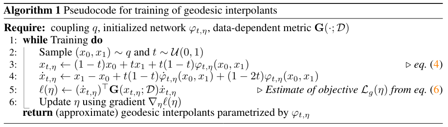
Geodesic interpolants learning

Once the RBF network has been trained on the empirical data to estimate its manifold, the network \(\psi_{t,\eta}\) is trained to rectify the interpolant following this algorithm:

 

Metric Flow Matching (MFM)

Now that we empirically know how to correct the straight trajectories to make them stay close to the data manifold, we can train our final network \(v_{t,\theta}\) to estimate the vector field following the new trajectories, with the loss:

\[\mathcal{L}_{\text{MFM}} = \mathbb{E}_{t, (x_0,x_1)\sim q} [ \lVert v_{t,\theta} (x_{t,\eta^*}) - \dot{x}_{t, \eta^*} \rVert^2 ]\]

From a technical point of view, the function jvc from PyTorch is used to compute the time derivatives of the output of the networks, such as \(\dot{\psi_{t,\eta}}\).

 

Experiments

The authors perform several experiments to validate the family of interpolants they build and their usefulness for MFM.

In Figure 2, we can observe that the learnt interpolants indeed allow to stay on each data manifold.

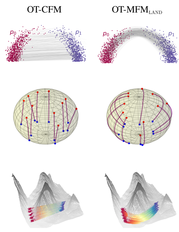
Figure 2. Interpolants learnt for three datasets.

 

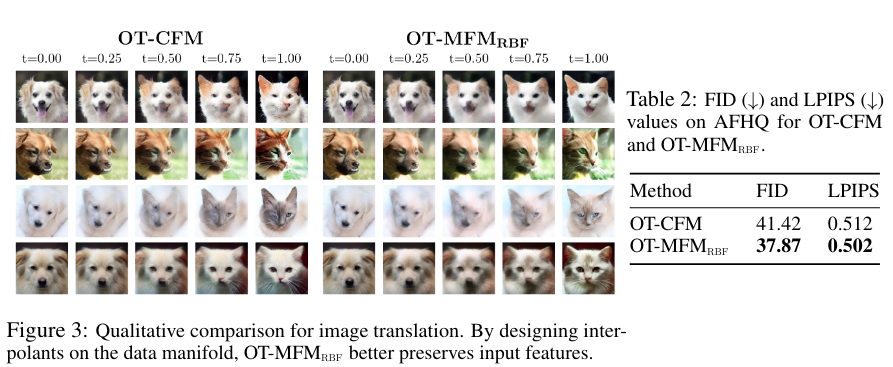
The authors performs unpaired data translation between dogs and cats from the dataset AFHQ in the latent space of the Stable Diffusion v1 VAE. Visual examples as well as quantitative comparison between their method (OT-MFM) and standard Flow Matching (OT-CFM) is provided below.

 

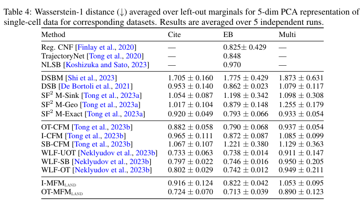
Finally, they test their model on the task of reconstructing cell dynamics, which is central in biomedical applications. Single-cell RNA sequencing is a destructive process, so their trajectories can not be tracked. We assume to have access to \(K\) unpaired distributions describing cell populations at \(K\) time points. The authors apply the MFM objective between every consecutive time points.

 

Conclusion

In this work, the authors propose a way to perform Flow Matching by following trajectories that stay close to an empirical data manifold. Contrary to previous related works, they have found a simulation-free approach, which make it scalable to large scale problems. I believe this work is really promising and will have significant applications to solve real-world problems in the future.