Understanding Contrastive Representation Learning through Alignment and Uniformity on the Hypersphere

Highlights

• Understanding the asymptotical behavior of the constrastive loss : both experimentally and theoretically.
• Proposes alternative losses that achieve the same or better performance on downstream tasks.

Introduction

In the context of unsupervised contrastive learning, positive pairs are defined as random transformations of the same input image. The objective is to bring these pairs closer in the representation space so that their embeddings become more similar. To achieve this, we rely on the contrastive loss, which encourages alignment of positive pairs while pushing apart negative ones. However, a central challenge lies in understanding the asymptotic behavior of the general contrastive loss.

\[\mathcal{L}_{\text{contrastive}}(f;\tau,M) \triangleq \underset{\substack{ (x,y)\sim p_{\text{pos}} \\ \{x_i^-\}_{i=1}^M \ \overset{\text{i.i.d.}}{\sim} p_{\text{data}} }}{\mathbb{E}} \left[ - \log \frac{ e^{f(x)^\top f(y)/\tau} } { e^{f(x)^\top f(y)/\tau} + \sum_i e^{f(x_i^-)^\top f(y)/\tau} } \right],\]

Motivation : In practice, only maximizing the Mutual Information (MI) (Kullback–Leibler divergence between the joint and the product of the marginal) between two views of the same image can result in poorer representations compared to using the contrastive loss ¹.

What the contrastive loss exactly does remains largely a mystery.

To address this, the authors propose to analyze the contrastive learning loss through two complementary properties: alignment and uniformity. They further validate these concepts empirically on standard representation learning benchmarks.

Intuition :

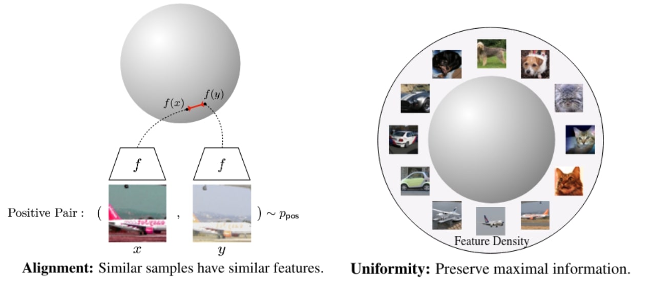
• Alignment : two similar samples should have the same representations.

• Uniformity : Empirically, normalizing features with an \(l_2\) norm improves performance (e.g., in face recognition) and stabilizes training. Moreover, when class features are sufficiently well clustered, they become linearly separable from the rest of the feature space.

Intuitively, pushing all features away from each other should indeed cause them to be roughly uniformly distributed.

Quantifying alignment and uniformity

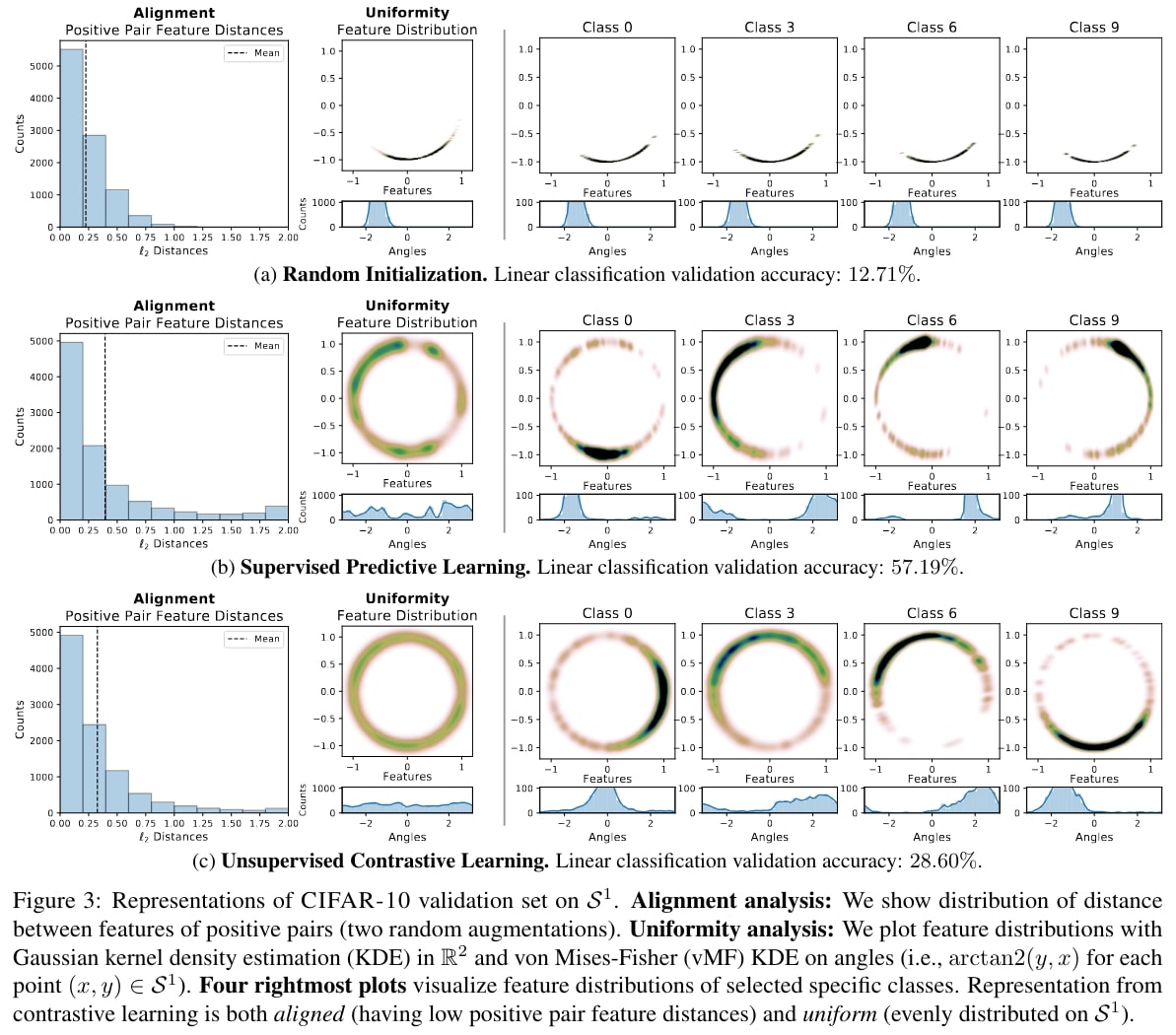
To quantify alignment, one can measure the distance between the representations of positive pairs: the closer they are, the better the alignment.

Quantifying uniformity is more subtle. The problem is related to the well-studied task of distributing points uniformly on the unit hypersphere, often formalized as minimizing the total pairwise potential with respect to a kernel function. Intuitively, this means we want the representations to be evenly spread out so that they balance each other, maintaining a sufficient distance to avoid collapse while covering the space effectively.

To empirically verify this, they used three encoders sharing the same AlexNet-based architecture modified to map input images to 2-dimensional vectors in \(\mathbb{S}^1\) on CIFAR-10 dataset:

• Random initialization.
• Supervised predictive learning: An encoder and a linear classifier are jointly trained from scratch with cross-entropy loss on supervised labels.
• Unsupervised contrastive learning: An encoder is trained w.r.t. \(\mathcal{L}_{\text{contrastive}}\) with \(\tau = 0.5\) and \(M = 256\).

Alternative losses

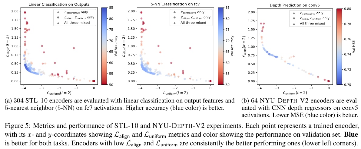
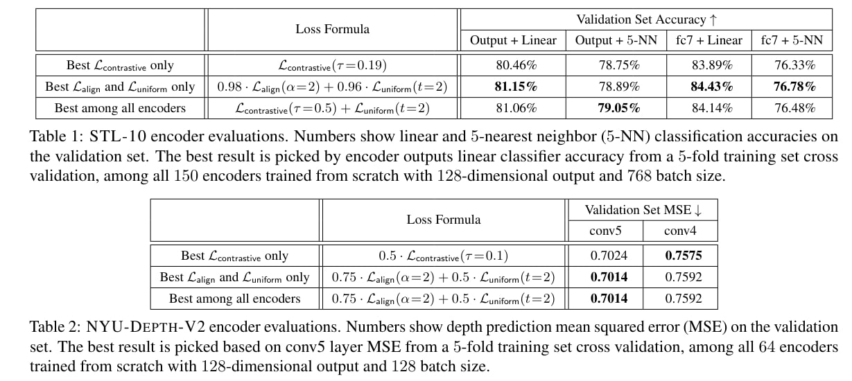
The article introduces two alternative losses, one capturing alignment and the other uniformity. The authors show, from a theoretical perspective, that contrastive loss implicitly optimizes both properties, and they characterize its asymptotic behavior. Empirically, they demonstrate that training directly with these two objectives achieves comparable, and in some cases superior, performance to standard contrastive loss.

Alignment loss : \(\mathcal{L}_{\text{align}}(f;\alpha) \triangleq \mathbb{E}_{(x,y)\sim p_{\text{pos}}} \left[ \| f(x) - f(y) \|_2^{\alpha} \right], \quad \alpha > 0.\)

Uniformity loss : Use the logarithm of the average pairwise Gaussian potential :

\[G_t(u, v) = e^{-t \|u-v\|^2_2} = e^{2t \cdot u^T v - 2t}, \quad t > 0,\]

defined as :

\[\mathcal{L}_{\text{uniform}}(f; t) = \log \mathbb{E}_{x, y \sim_{\text{i.i.d.}} p_{\text{data}}} \big[ G_t(u, v) \big] = \log \mathbb{E}_{x, y \sim_{\text{i.i.d.}} p_{\text{data}}} \big[ e^{-t \| f(x) - f(y) \|_2^2} \big], \quad t > 0.\]

Proposition.
For \(M(S^d)\), the set of Borel probability measures on \(S^d\), \(\sigma_d\) (e.g. normalized surface area measure on \(S^d\)) is the unique solution of:

\[\sigma_d = \underset{\mu \in M(S^d)}{\arg\min} \int_{u} \int_{v} G_t(u, v) \, d\mu(u) \, d\mu(v)\]

As number of points goes to infinity, distributions of points minimizing the average pairwise potential converge weak to the uniform distribution. “Due to its pairwise nature, \(L_{\text{uniform}}\) is much simpler in form and avoids the computationally expensive softmax operation in \(L_{\text{contrastive}}\).”

Theorem 1 (Asymptotics of \(L_{\text{contrastive}}\)).
For fixed \(\tau > 0\), as the number of negative samples \(M \to \infty\), the (normalized) contrastive loss converges to

\[\lim_{M \to \infty} \; L_{\text{contrastive}}(f; \tau, M) - \log M = -\frac{1}{\tau} \; \mathbb{E}_{(x,y) \sim p_{\text{pos}}} \big[ f(x)^\top f(y) \big] + \mathbb{E}_{x \sim p_{\text{data}}} \left[ \log \; \mathbb{E}_{x^- \sim p_{\text{data}}} \big[ e^{f(x^-)^\top f(x) / \tau} \big] \right].\]

We have the following results:

1. The first term is minimized iff \(f\) is perfectly aligned.
2. If perfectly uniform encoders exist, they are the exact minimizers of the second term.
3. For the convergence of the equation above, the absolute deviation from the limit decays as \(\mathcal{O}(M^{-1/2})\).

Experiments

They conducted their experiments on multiple representation learning tasks :

• STL-10 classification on AlexNet based encoder outputs or intermediate activations with a linear or k-nearest neighbor (k-NN) classifier.
• NYU-DEPTH-V2 depth prediction on CNN encoder intermediate activations after convolution layers.
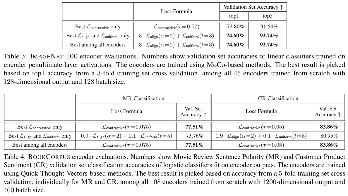
• IMAGENET and IMAGENET-100 (random 100-class subset of IMAGENET) classification on CNN encoder penultimate layer activations with a linear classifier.
• BOOKCORPUS RNN sentence encoder outputs used for Moview Review Sentence Polarity (MR) and Customer Product Review Sentiment (CR) binary classification tasks with logisitic classifiers (positive pairs are chosen as neighboring sentences, following Quick-Thought Vectors).

Limitations

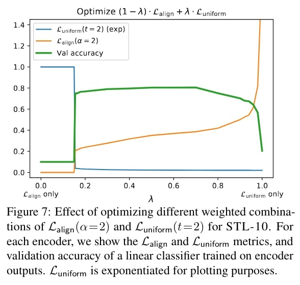
The trade-off between the \(L_{\text{align}}\) and \(L_{\text{uniform}}\) indicates that perfect alignment and perfect uniformity are likely hard to simultaneously achieve in practice. However, the inverted-U shaped accuracy curve confirms that both properties are indeed necessary for a good encoder.

References

1. Tschannen, M., Djolonga, J., Rubenstein, P. K., Gelly, S., and Lucic, M. On mutual information maximization for representation learning (2019). arXiv:1907.13625. ↩