Notes

Link to the code here

VAE reminders

The full presentation, including links to the diffusion model (DDPM), is available here

Highlights

Develop a deep unsupervised probabilistic approach for hierarchical clustering
Extension of VAE framework to tree-based posterior distribution over latent variables
Complex distributions are approximated through Monte Carlo techniques
Integration of a contrastive loss to reinforce accurate and contextually meaningfull clustering
Evaluation from several public datasets: MNIST, Fashion-MNIST, 20Newsgroups and Omniglot-5

Model architecture / design strongly inspired by decision trees

Motivations

Unsupervised clustering model expression through deep learning paradigm

Overall idea

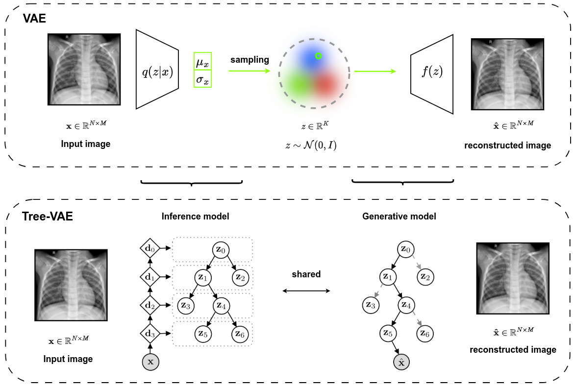
In standard VAE, the same decoder reconstructs all the images of the training dataset
This can lead to difficulties in terms of reconstruction accuracy

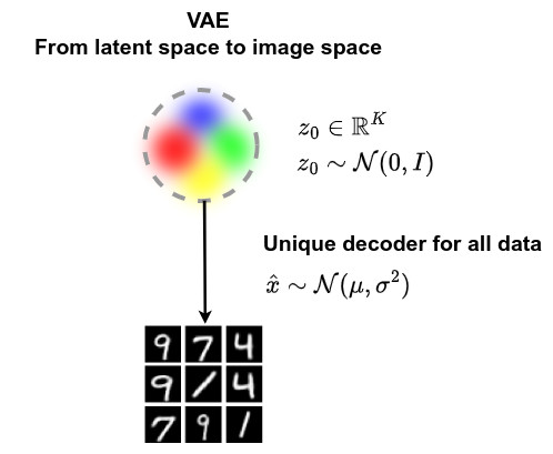
In treeVAE, multiple decoders are used to reconstruct the training images per group
Optimizing reconstruction quality may lead to image groups sharing similar properties, thereby forming clusters

Methodology

Overall architecture

Analogy with the classical VAE

Generation of the binary tree \(\mathcal{T}\)

During training, the structure of the tree needs to be fixed.
Design an iterative process to automatically generate a tree in an unsupervised manner

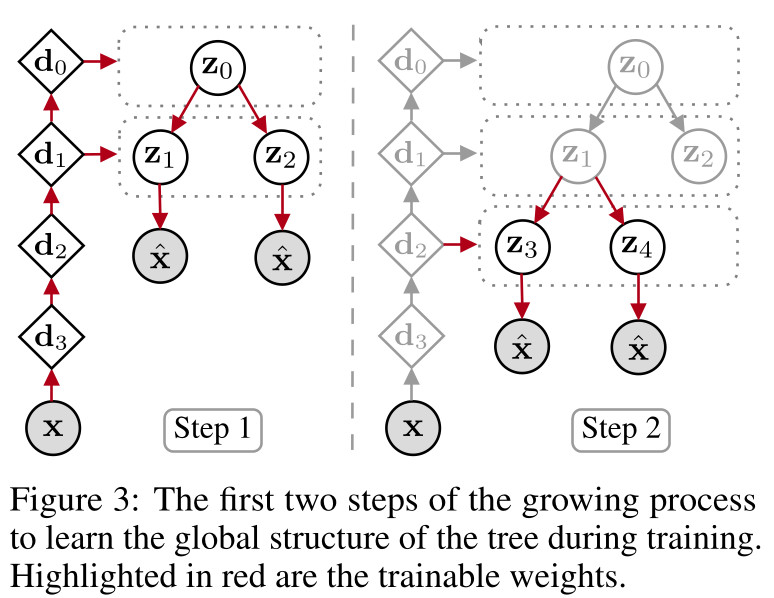
Predefine the maximum depth (in this example 4)
Training a tree composed of a root and two leaves for \(N_t\) epochs by optimizing the ELBO
Once the model converged, a leaf is selected and two children are attached to it. The leaf criteria can vary according to the application. In these experiments, the authors chose to select the nodes with the number of samples higher than a threshold to retain balanced leaves
The sub-tree composed of the new leaves and the parent node is then trained for \(N_t\) epochs by freezing the weights of the rest of the model and by optimizing the ELBO. At this stage, the sub-tree is trained using only the subset of data that have a high probability (higher than a threshold) of being assigned to the parent node
The process is repeated until the tree reaches its maximum depth or until a condition (e.g. predefined maximum number of leaves) is met
The entire model is then fine-tuned for \(N_f\) epochs by unfreezing all weights. During this stage, the tree is pruned by removing almost empty branches (with the expected number of assigned samples lower than a threshold)

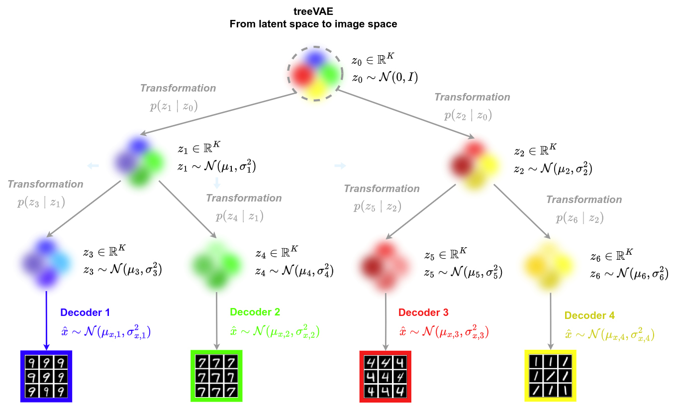
Generative model

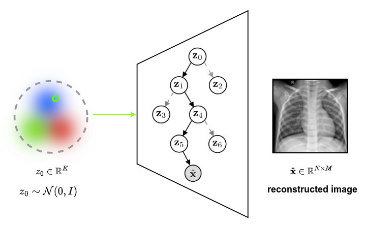
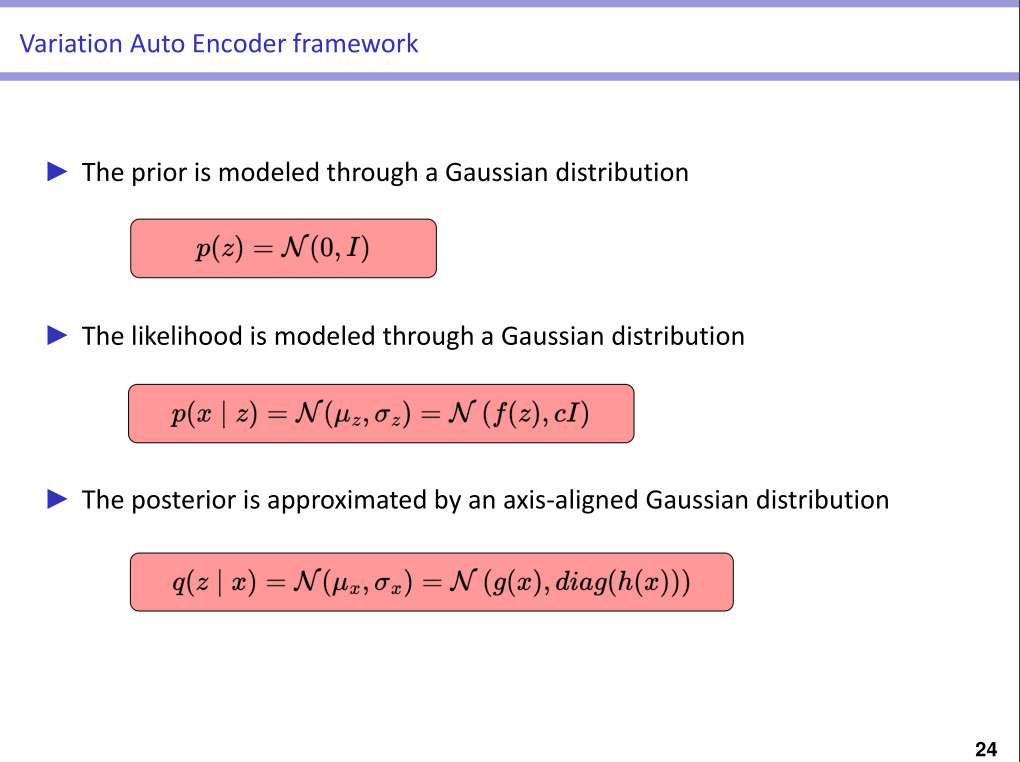
The latent embedding of the root node \(z_0\) is sample from a standard Gaussian \(z_0 \sim \mathcal{N}\left( 0, I \right)\)
The decision of going on the left or the right node is sampled from a Bernoulli distribution \(p(c_0 \mid z_0) = Ber(r_{p,0}(z_0))\) where \(\{r_{p,i} \mid \, i \in \mathbb{V} \, \backslash \, \mathbb{L} \}\) are functions parametrized by neural networks (simple MLP with two hidden layers with 128x2 neurons + leaky ReLU ) defined as routers. \(\mathbb{V}\) is the set of nodes and \(\mathbb{L}\) is the set of leaves.

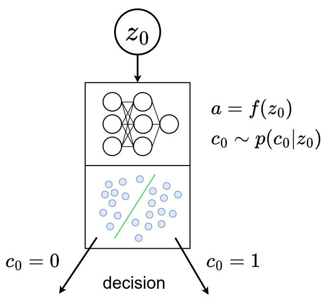
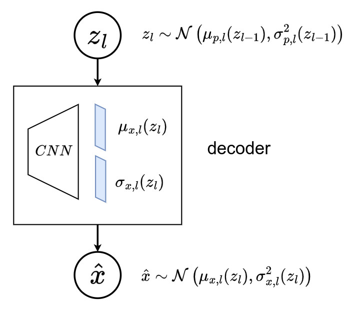
The latent embedding of the selected child, e.g. \(z_1\), is then sampled from a Gaussian distribution \(z_1 \sim \mathcal{N}\left( \mu_{p,1}(z_0), \sigma^2_{p,1}(z_0) \right)\), where \(\{ \mu_{p,i}, \sigma_{p,i} \, \mid i \in \mathbb{V} \, \backslash \, \{0\} \}\) are functions parametrized by neural networks defined as transformations.

This process continues until a leaf is reached
➔ \(z_{\mathcal{P}_l} = \{ z_i \mid i \in \mathcal{P}_l \}\) the set of latent variables selected by the path \(\mathcal{P}_l\), which goes from the root to the leaf \(l\)
➔ \(pa(i)\) the parent node of the node \(i\)
➔ \(p(c_{pa(i) \to i} \mid z_{pa(i)})\) the probability of going from \(pa(i)\) to \(i\)
➔ \(\mathcal{P}_l\) defines the sequence of decisions
The prior probability of the latent embeddings and the path given \(\mathcal{T}\) can be summarized as:
➔ \(p_{\theta}(z_{\mathcal{P}_l}, \mathcal{P}_l) = p(z_0) \, \prod_{i\in \mathcal{P}_l \backslash \{0\}}{\, \, \underbrace{p(c_{pa(i) \to i} \mid z_{pa(i)})}_{\text{path}} \, \cdot \, \underbrace{p(z_i \mid z_{pa(i)})}_{\text{latent variable}}}\)
Finally, \(x\) is sampled from a distribution that is conditionned on the selected leaf \(p_{\theta}(x \mid z_{\mathcal{P}_l}, \mathcal{P}_l) = \mathcal{N}(\mu_{x,l}(z_l), \sigma_{x,l}^2(z_l))\), where \(\{ \mu_{x,l} , \sigma_{x,l} \mid l \in \mathbb{L}\}\) are functions parametrized by leaf-specific neural networks defined as decoders

Inference model

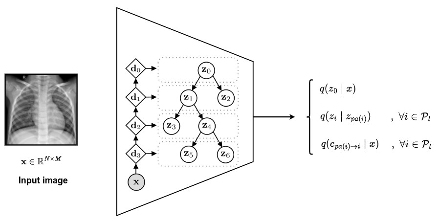
Described by the variational posterior distribution of both the latent embeddings \(z_{\mathcal{P}_l}\) and the paths \(\mathcal{P}_l\)
The probability of the root and of the decisions are now conditioned on the sample \(x\)
➔ \(q(z_{\mathcal{P}_l}, \mathcal{P}_l \mid x) = q(z_0 \mid x) \, \prod_{i\in \mathcal{P}_l \backslash \{0\}}{\, \, \underbrace{q(c_{pa(i) \to i} \mid x)}_{\text{path}} \, \cdot \, \underbrace{q(z_i \mid z_{pa(i)})}_{\text{latent variable}}}\)
The authors used the work of Sonderby et al. to compute the variational probability distribution of the latent embeddings \(q(z_0 \mid x)\) and \(q(z_i \mid z_{pa(i)})\)
➔ \(q(z_0 \mid x) = \mathcal{N}( \mu_{q,0}(x), \sigma^2_{q,0}(x) )\)
➔ \(q(z_i \mid z_{pa(i)}) = \mathcal{N}( \mu_{q,i}(z_{pa(i)}), \sigma^2_{q,i}(z_{pa(i)}) ) \,\), \(\, \forall i \in \mathcal{P}_l\)
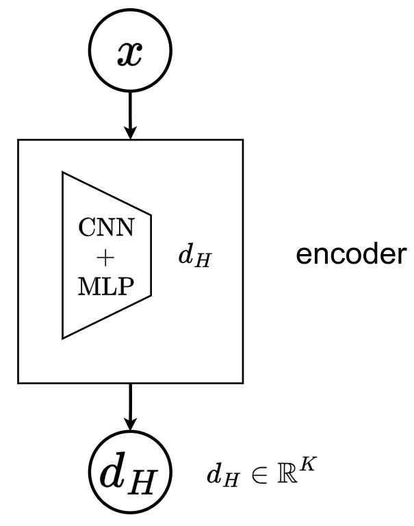
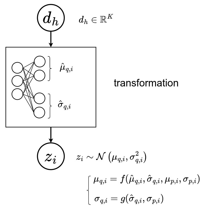
First, a deterministic a bottom-up pass computes the node-specific approximate contributions:
➔ \(d_h = \text{MLP}(d_{h+1})\)
➔ \(\hat{\mu}_{q,i} = \text{Linear}(d_{depth(i)}) \,\), \(\, i \in \mathbb{V}\)
➔ \(\hat{\sigma}^2_{q,i} = \text{Softplus}(\text{Linear}(d_{depth(i)})) \,\), \(\, i \in \mathbb{V}\)
➔ where \(d_H\) is parametrized by a domain-specific neural network defined as encoder

➔ \(\text{MLP}(d_h)\) for \(h \in \{1,\cdots,H\}\) are neural networks shared among the parameter predictors, \(\hat{\mu}_{q,i}, \hat{\sigma}^2_{q,i}\) at the same depth
➔ they are characterized by the same architecture as the transformations used in the generative model

A stochastic downward pass then recursively computes the approximate posteriors
➔ \(\sigma^2_{q,i} = \frac{1}{ \hat{\sigma}^{-2}_{q,i} \, + \, \sigma^{-2}_{p,i} }\)
➔ \(\mu_{q,i} = \frac{ \hat{\mu}_{q,i} \, \cdot \, \hat{\sigma}^{-2}_{q,i} \,+\, \mu_{p,i} \, \cdot \, \sigma^{-2}_{p,i} }{ \hat{\sigma}^{-2}_{q,i} \, + \, \sigma^{-2}_{p,i} }\)

Finally, the variational distributions of the decisions \(q(c_i \mid x)\) are defined as
➔ \(q(c_i \mid x) = q(c_i \mid d_{\text{depth(i)}}) = Ber(r_{q,i}(d_{\text{depth(i)}}))\)
➔ where \(\{ r_{q,i} \, \mid \, i \in \mathbb{V} \, \backslash \, \mathbb{L} \}\) are functions parametrized by neural networks and are characterized by the same architecture as the routers of the generative model

Learning process

The parameters of both the generative model (defined as \(p\)) and inference model (defined as \(q\)), consisting of the encoder \((\mu_{q,0}, \sigma_{q,0})\), the transformations (\(\{ (\mu_{p,i},\sigma_{p,i}), (\mu_{q,i},\sigma_{q,i}) \, \mid \, i \in \mathbb{V} \backslash \{0\} \}\)), the decoders (\(\{ \mu_{x,l}, \sigma_{x,l} \, \mid \, l \in \mathbb{L} \}\)) and the routers (\(\{ r_{p,i}, r_{q,i} \, \mid \, i \in \mathbb{V} \, \backslash \, \mathbb{L} \}\)) are learned by maximizing the ELBO
Each leaf \(l\) is associated with only one path \(\mathcal{P}_l\). The data likelihood conditioned on \(\mathcal{T}\) can be written as:
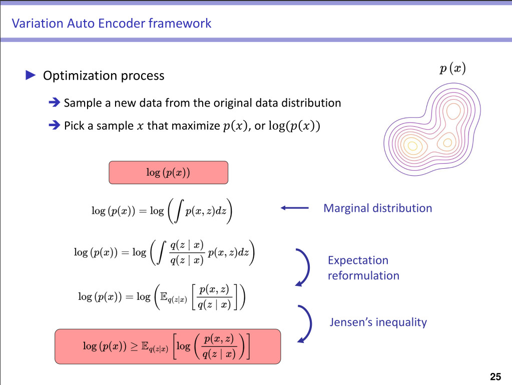
➔ \(p(x \mid \mathcal{T}) = \sum_{l \in \mathbb{L}}{\int_{z_{\mathcal{P}_l}}}{p(x,z_{\mathcal{P}_l},\mathcal{P}_l)} \, \,\) (use of the of the marginal)
➔ \(p(x \mid \mathcal{T}) = \sum_{l \in \mathbb{L}}{\int_{z_{\mathcal{P}_l}}}{p_{\theta}(z_{\mathcal{P}_l}, \mathcal{P}_l) \, \cdot\, p_{\theta}(x \mid z_{\mathcal{P}_l},\mathcal{P}_l)} \, \,\) (use of the of Bayes’ formula)
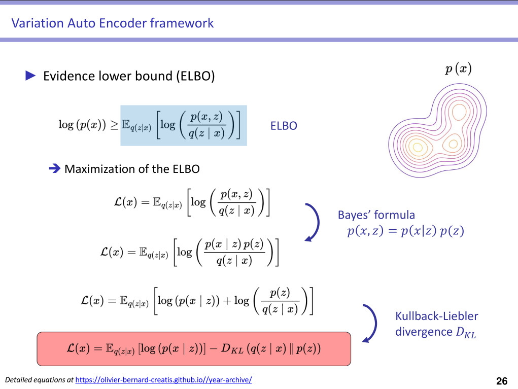
Use variational inference to derive the ELBO of the log-likelihood
➔ \(\mathcal{L}(x \mid \mathcal{T}) := \underbrace{\mathbb{E}_{q(z_{\mathcal{P}_l},\mathcal{P}_l \mid x)}[ \text{log} \, p(x \mid z_{\mathcal{P}_l},\mathcal{P}_l) ]}_{\text{data fidelity}} \, - \, \underbrace{\text{KL}(q(z_{\mathcal{P}_l},\mathcal{P}_l \mid x) \parallel p(z_{\mathcal{P}_l},\mathcal{P}_l) )}_{\text{distributions fit}}\)
See paper for all the derivations ;)
➔ Use of Monte Carlo framework to estimate some distributions !

Data fidelity term

The data fidelity term can be expressed as:
➔ \(\mathcal{L}_{rec} = \mathbb{E}_{q(z_{\mathcal{P}_l},\mathcal{P}_l \mid x)}[ \text{log} \, p(x \mid z_{\mathcal{P}_l},\mathcal{P}_l) ]\)
➔ \(\mathcal{L}_{rec} \approx \frac{1}{M} \sum_{m=1}^{M} \sum_{l\in \mathbb{L}}{P(l;c)\log (\mathcal{N(\mu_{x,l}(z_l^{(m)}),\sigma_{x,l}^2(z_l^{(m)})))}}\)
- with \(P(i;c)=\prod_{j\in P_{i \backslash \{0\}}}q(c_{pa(j) \rightarrow j} \mid x)\) for \(i \in \mathbb{V}\) the probability of reaching node \(i\), which corresponds to the product over the probabilities of the decisions in the path until \(i\)
- with \(z_l^{(m)}\) the Monte Carlo (MC) samples, and \(M\) the number of MC samples.

Distributions fit term

The distributions fit term can be expressed as:
➔ \(\text{KL}(q(z_{\mathcal{P}_l},\mathcal{P}_l \mid x) \parallel p(z_{\mathcal{P}_l},\mathcal{P}_l) ) = \text{KL}_{root} + \text{KL}_{nodes} + \text{KL}_{decisions}\)
➔ \(\text{KL}_{root} = \text{KL}(q(z_0 \mid x) \parallel p(z_0))\)
➔ \(\text{KL}_{nodes} \approx \frac{1}{M} \sum_{m=1}^{M} \sum_{i \in \mathbb{V} \backslash \{0\}} P(i;c) \, \text{KL}(q(z_i^{(m)} \mid pa(z_i^{(m)})) \parallel p(z_i^{(m)} \mid pa(z_i^{(m)})))\)
➔ \(\text{KL}_{decisions} \approx \frac{1}{M} \sum_{m=1}^{M} \sum_{i \in \mathbb{V} \backslash \{\mathbb{L}\}} P(i;c) \, \text{KL}(q(c_i \mid x) \parallel p(c_i \mid z_i))\)

Experiments

Evaluation on 8 public datasets (small images): MNIST, Fashion-MNIST, 20Newsgroups, Omniglot, Omniglot-5, CIFAR-10 and CIFAR-100, CelebA
Comparison with baseline methods: VAE (non-hierarchical method) and LadderVAE (sequential method)
The dimension of all latent embeddings \(z = \{z_0, \cdots, z_V \}\) is the same and is equal to 8 for MNIST, Fashion, and Omniglot, to 4 for 20Newsgroups, and to 64 for CIFAR-10, CIFAR-100, and CelebA
The maximum depth of the tree is set to 6 for all datasets, except 20Newsgroups where depth was increased to 7 to capture more clusters
To compute DP and LP, the tree is allowed to grow to a maximum of 30 leaves for 20Newsgroups and CIFAR-100, and 20 for the rest, while for ACC and NMI the number of leaves is set to the number of true classes
The transformations consist of one-layer MLPs of size 128 and the routers of two-layers of size 128 for all datasets except for the real-world imaging data where the size of the MLP is increased to 512
the encoder and decoders consist of simple CNNs and MLPs
The trees are trained for \(N_t = 150\) epochs at each growth step, and the final tree is finetuned for \(N_f = 200\) epochs
All experiments were run on RTX3080 GPUs
Training TreeVAE with 10 leaves on MNIST, Fashion-MNIST, and Omniglot-50 takes between 1h and 2h, Omniglot-5 30 minutes, CIFAR-10 5h
Training TreeVAE with 20 leaves on 20Newsgroup takes approximately 30 minutes, and on CIFAR-100 9h
Training TreeVAE on CelebA takes approx 8h

Results

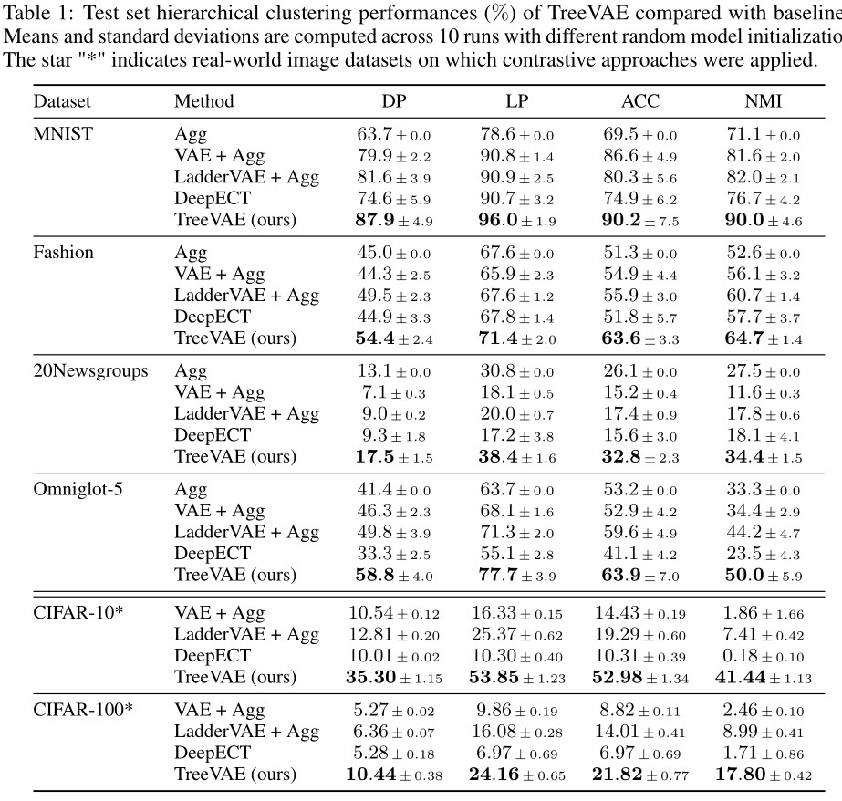
Clustering performances

Assessement of the hierarchical clustering performance by computing dendrogram purity (DP) and leaf purity (LP), , as defined by Kobren et al., and the more standard clustering metrics: accuracy (ACC) and normalized mutual information (NMI), by setting the number of leaves for TreeVAE and for the baselines to the true number of clusters

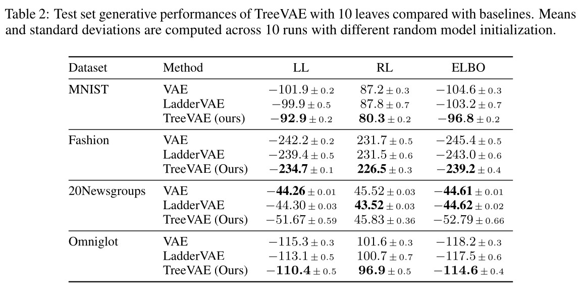
Generative capacities

Compute the approximated true log-likelihood (LL) calculated using 1000 importance-weighted samples, together with the ELBO and the reconstruction loss (RL)

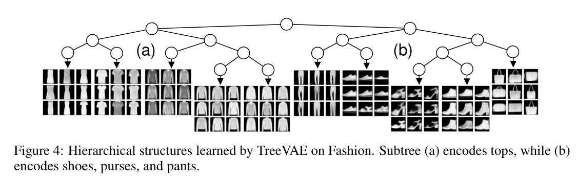
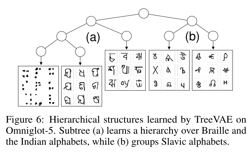
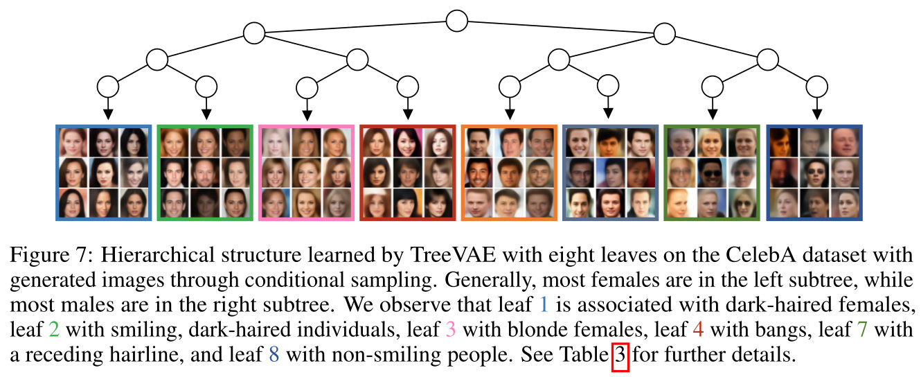
Discovery of Hierarchies

In addition to solely clustering data, TreeVAE is able to discover meaningful hierarchical relations between the clusters, thus allowing for more insights into the dataset

Conclusions

This paper presents an unsupervised clustering-based VAE method
The model architecture / design is strongly inspired by decision trees
Results vary with key parameters (max number of leafs, depth, different thresholds) that need to be manually selected
The method seems computationally expensive