KAN: Kolmogorov–Arnold Networks
Highlights
- Kolmogorov–Arnold Networks (KANs) are proposed as a promising alternative to Multi-Layer Perceptrons (MLPs).
- Every weight parameter in a KAN is replaced by a univariate function parameterized as a spline, meaning activation functions are learnable and placed on the edges (“weights”) instead of fixed on the nodes (“neurons”).
- KANs offer superior interpretability compared to MLPs, particularly for small-scale AI + Science tasks, facilitating the (re)discovery of mathematical and physical laws.
- They demonstrate better accuracy and possess faster neural scaling laws (NSLs) than MLPs.
- The corresponding code is available on the official GitHub repository.
Introduction
Introduction and MLP Reminder
Multi-Layer Perceptrons (MLPs)
- Positive Point :
- MLP are the fundamental building blocks of most modern deep learning models, their expressive power guaranteed by the Universal Approximation Theorem
- Negative Point :
- less intepretable
- need to retrain MLPs if it’s not adapted to dataset
Kolmogorov-Arnold Network
- Positive Point :
- based on Kolmogorov-Arnold Representation theorem: they established that if f is a multivariate continuous function, then f can be written as a finite composition of continuous functions of a single variable and the binary operation of addition.
- can change the finesse of the network after training
- typically require a much smaller computational graph (fewer neurons and layers) than MLPs.
Motivation: Overcoming MLP and Spline Limitations
KANs are designed to integrate the best qualities of both splines and MLPs.
Splines are highly accurate for low-dimensional functions and offer local adjustability, but they suffer severely from the Curse of Dimensionality (COD) because they cannot exploit compositional structures. Conversely, MLPs are less affected by COD due to their feature learning capabilities, but they are often less accurate than splines when approximating simple univariate functions in low dimensions.
The standard Universal Approximation Theorem, which justifies MLPs, itself struggles with COD, suggesting that the number of required neurons can grow exponentially with input dimension \(d\). The authors show that KANs combine MLPs on the exterior (to learn compositional structure) and splines on the interior (to accurately approximate univariate functions). Theoretically, KANs can beat the COD if the target function admits a smooth Kolmogorov-Arnold representation.
B-Spline
3 hyperparameters :
- n : polynome degrees
- m+1 : number of nodes \((t_0, ..t_m)\) \(0 \leq t_0 \leq t_1 \leq \dots \leq t_m \leq 1\) (call grid in KAN)
- \(P_i\) : control polynomial, the number of control points is equal to m-n
The B-spline definition sets: \(\mathbf{S} : [0, 1] \to \mathbb{R}^d\)
The curve is defined by \(\mathbf{S}(t) = \sum_{i=0}^{m-n-1} b_{i,n}(t) \, \mathbf{P}_i, \quad t \in [t_n, t_{m-n}]\). The m-n degree B-spline functions are defined by recurrence (Cox-de Boor recurrence) on the lower degree: \(b_{j,0}(t) := \begin{cases} 1 & \text{if } t_j \leq t < t_{j+1} \\ 0 & \text{else} \end{cases}\)
\[b_{j,n}(t) := \frac{t - t_j}{t_{j+n} - t_j} b_{j,n-1}(t) + \frac{t_{j+n+1} - t}{t_{j+n+1} - t_{j+1}} b_{j+1,n-1}(t)\]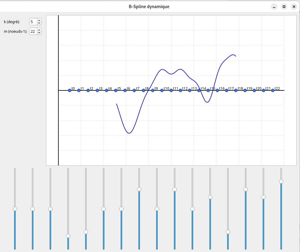
Figure 1. B-Spline 1D illustration .
Kolmogorov–Arnold Networks (KAN)
The KAN architecture generalizes the original Kolmogorov–Arnold representation (a fixed depth-2, width-(2n+1) structure) to arbitrary widths and depths.
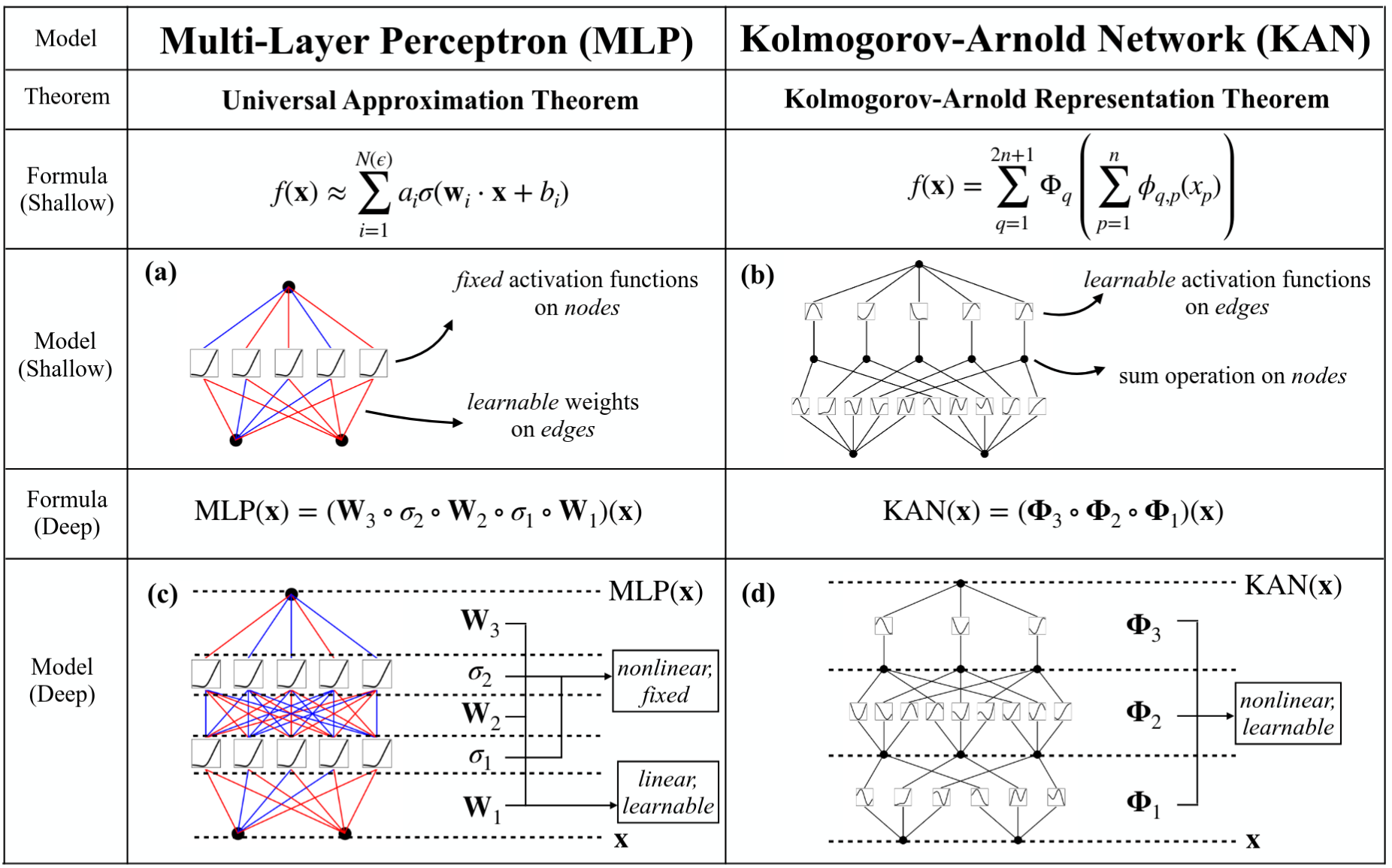
Figure 2. Multi-Layer Perceptrons (MLPs) vs. Kolmogorov-Arnold Networks (KANs) .
KAN Architecture
In a KAN, nodes perform a simple summation of incoming signals without applying any non-linearity. The activation of the \(j\)-th neuron in layer \(l+1\), \(x_{l+1,j}\), is defined as the sum of the post-activations of the univariate functions \(\phi_{l,j,i}\) applied to the inputs \(x_{l,i}\): \(x_{l+1,j} = \sum_{i=1}^{n_l} \phi_{l,j,i}(x_{l,i})\)
Each activation function \(\phi(x)\) is parameterized as a sum of a basis function \(b(x)\) and a B-spline function:
\(\phi(x) = w_b b(x) + w_s \text{spline}(x)\)
where \(b(x)\) is typically the SiLU function (\(b(x) = x / (1 + \exp^{-x})\)).
\(w_b\), \(w_s\) and B-spline control points are the parameters that are learned during training.
Approximation Capabilities and Scaling Laws
Theorem (Approximation theory, Kolmogorov-Arnold Theorem). Let \(\mathbf{x} = (x_1, x_2, \dots, x_n)\). Suppose that a function \(f(\mathbf{x})\) admits a representation
\[f = (\Phi_{L-1} \circ \Phi_{L-2} \circ \cdots \circ \Phi_1 \circ \Phi_0) \mathbf{x}\]as in, where each one of the \(\Phi_{l,i,j}\) are \((k+1)\)-times continuously differentiable. Then there exists a constant \(C\) depending on \(f\) and its representation, such that we have the following approximation bound in terms of the grid size \(G\): there exist \(k\)-th order B-spline functions \(\Phi_{l,i,j}^G\) such that for any \(0 \leq m \leq k\), we have the bound
\[\| f - (\Phi_{L-1}^G \circ \Phi_{L-2}^G \circ \cdots \circ \Phi_1^G \circ \Phi_0^G) \mathbf{x} \|_{C^m} \leq C G^{-k-1+m}\]Accuracy : Grid extension
-
have a finer grid from \(\{t_0,t_1,...,t_{G_1}\}\) to \(\{t_{-k},...,t_{-1},t_0,...,t_{G_1},t_{G_1+1},...,t_{G_1+k}\}\)
-
KAN can start training with fewer parameter, then extend it
-
Small KAN generalizes better
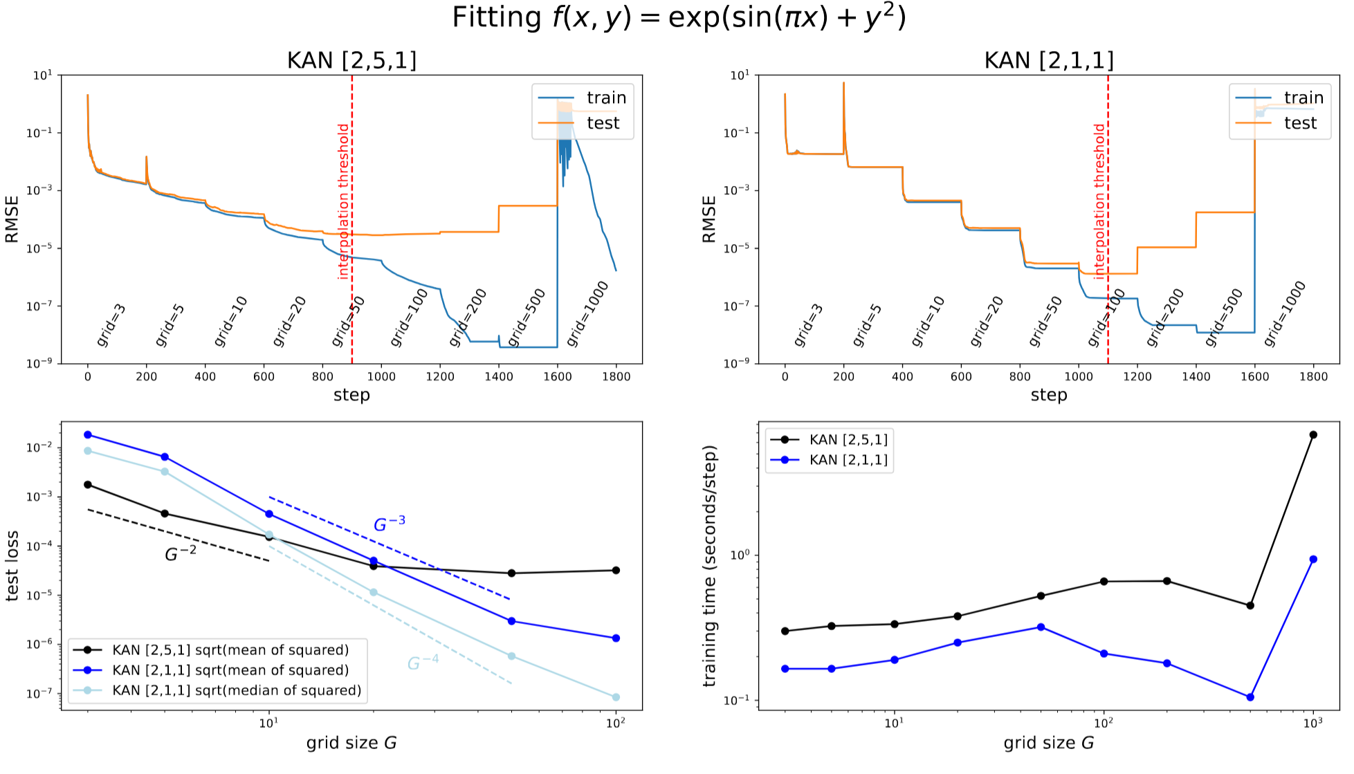
Figure 3. We can make KANs more accurate by grid extension (fine-graining spline grids). Top left (right): training dynamics of a [2, 5, 1] ([2, 1, 1]) KAN. Both models display staircases in their loss curves, i.e., loss suddently drops then plateaus after grid extension. Bottom left: test RMSE follows scaling laws against grid size G. Bottom right: training time scales favorably with grid size G.
Simplifying KANs and Making them interactive
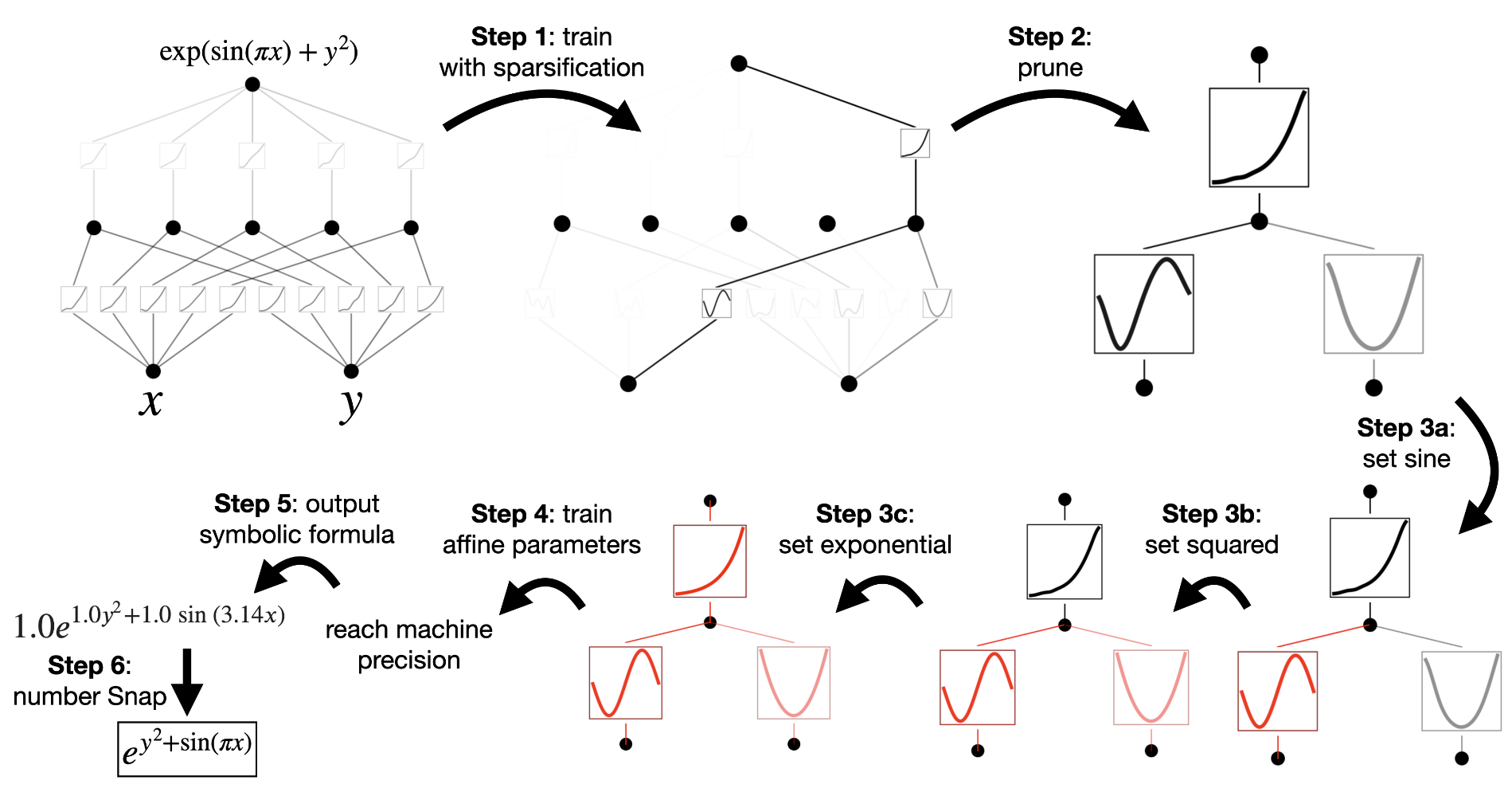
Figure 4. An example of how to do symbolic regression with KAN.
- Visualise: check magnitude of activation function \(\| \phi \|_{1} \equiv \frac{1}{N_p} \sum_{s=1}^{N_p} \| \phi(x^{(s)}) \|\)
- Prune: delete activation functions with less importance
- Symbolification: if the activation function resembles a known function, it can be replaced.(ex: y = cf(ax+b)+d)
Discussion
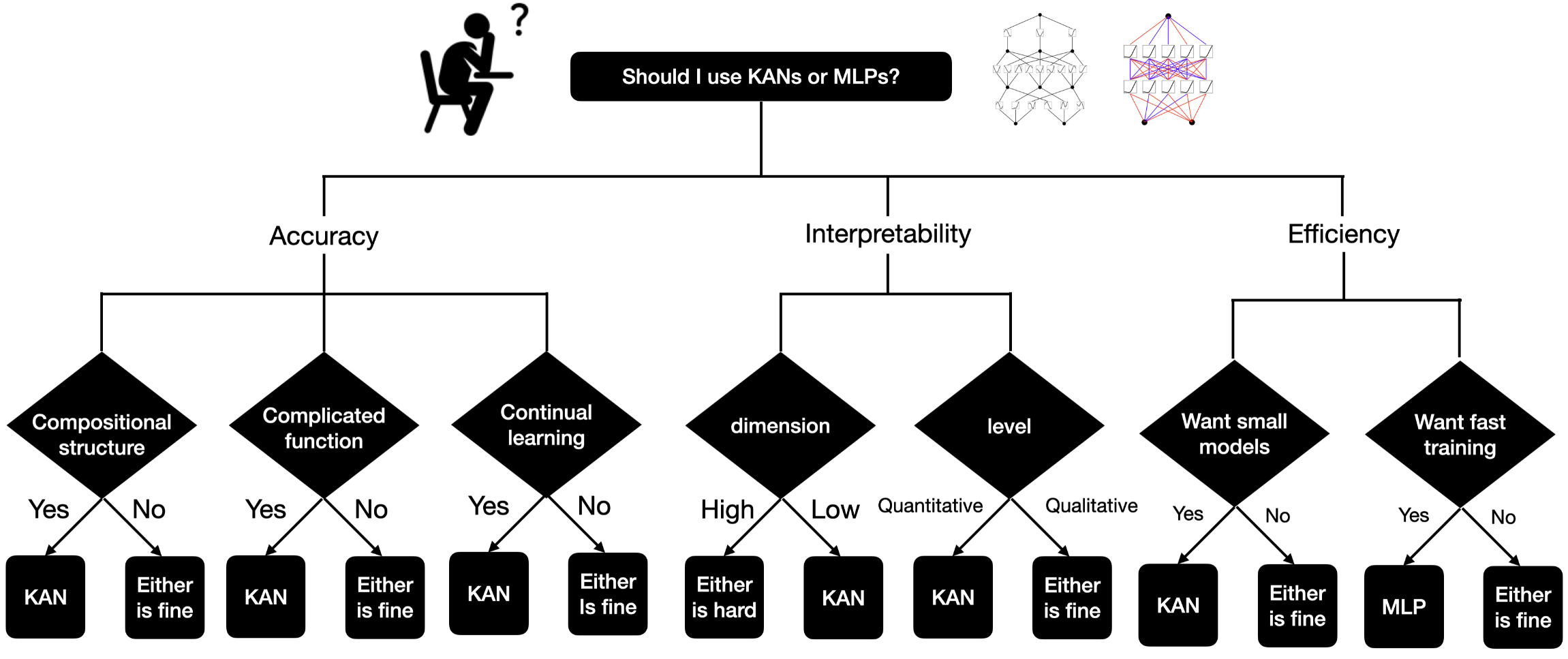
Figure 5. Should I use KANs or MLPs?.
- B-Spline is set only between 0 and 1. How did they handle it ?