MAD-AD: Masked Diffusion for Unsupervised Brain Anomaly Detection
Notes
- Link to the code here
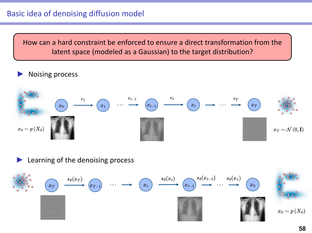
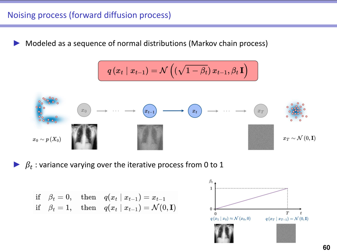
Diffusion model reminders
The full presentation, including links to the diffusion model (DDPM), is available here
Highlights
- Extending the idea proposed in the THOR method 1 to the training procedure
- Learning to remove regions with anomalies of varying sizes using a diffusion process
- Evaluation on three public datasets:
IXI Dataset(brain MRI scans from approximately 600 healthy subjects),ATLAS 2.0(655 T1-weighted MRI scans accompanied by expert-segmented lesion masks), andBraTS'21(1251 brain scans across four modalities: T1-weighted, contrast-enhanced T1-weighted - T1CE, T2-weighted, and T2 Fluid Attenuated Inversion Recovery - FLAIR)
Motivations
- Removing the need for forward and reverse processes in diffusion-based anomaly detection avoids several limitations, including feature degradation during forward diffusion and a trade-off between localization accuracy and removable anomaly size.
Overall idea
- The method is based on the following hypothesis: starting from a VAE trained exclusively on normal subjects, a region containing abnormalities is efficiently represented as noise in the corresponding latent space.
- Using a dataset of healthy subjects, relevant synthetic anomalies can be introduced by adding Gaussian noise of varying intensity to randomly selected regions via a forward diffusion process, and subsequently learning to remove them through a reverse diffusion process.
Key ideas
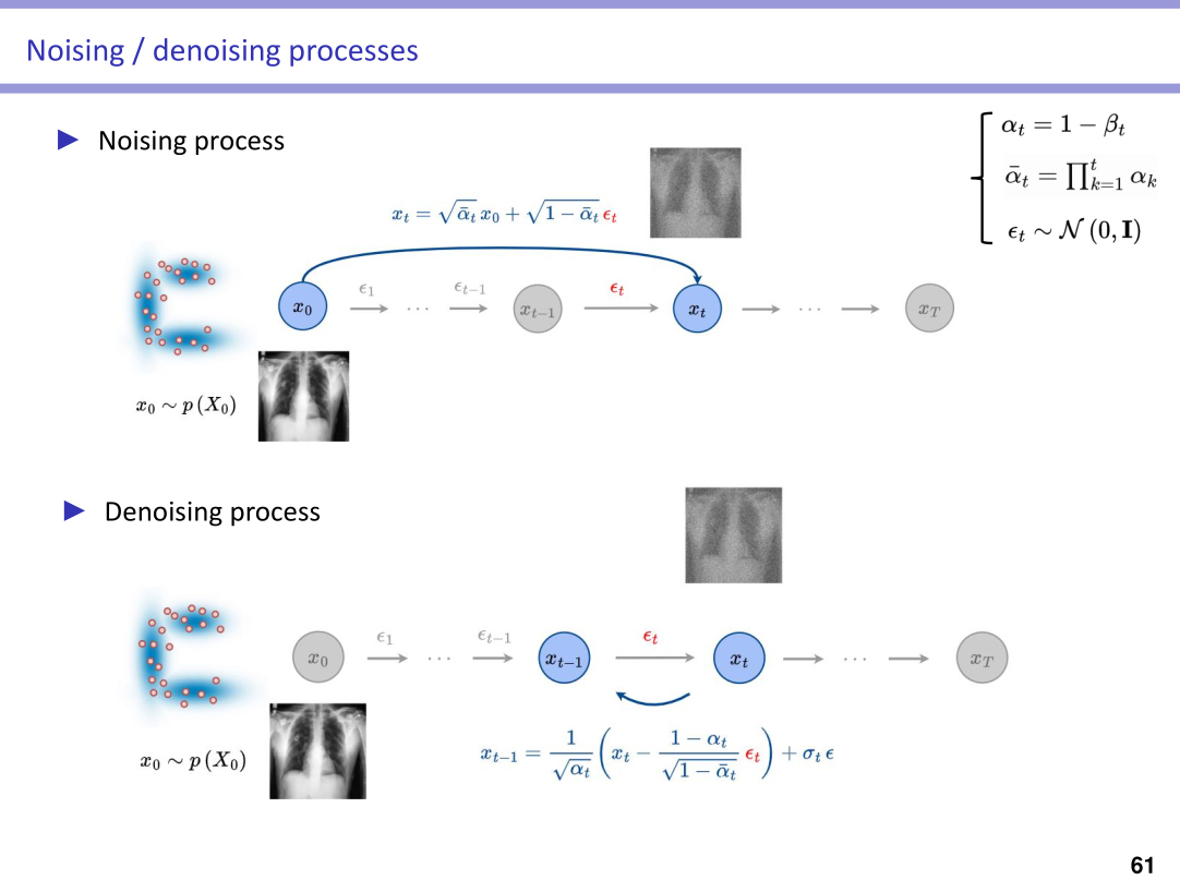
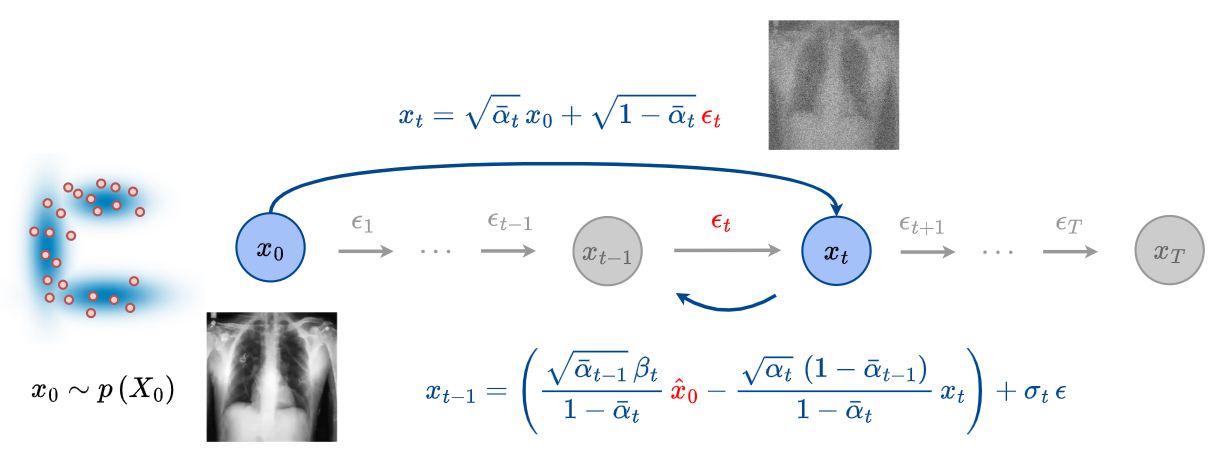
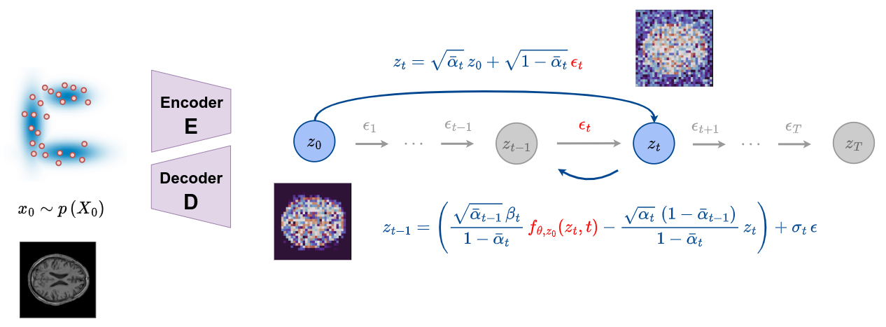
- The diffusion process can be revisited by estimating \(x_0\), denoted as \(\hat{x}_0\), at any time step \(t\) using the following equations.
DDPM
- Computation of the estimated \(\hat{x}_0(x_t,t)\) from \(\epsilon_\theta(x_t,t)\)
- Computation of \(\epsilon_\theta(x_t,t)\) from the estimated \(\hat{x}_0(x_t,t)\)
- The reverse process that links \(x_{t-1}\) with \(x_t\) can be rewritten as:
DDIM
- DDIM is commonly used to reconstruct images through a deterministic sampling process
- The following DDIM expression is always true:
- Using the relation that links \(\epsilon_{\theta}\) with \(\hat{x}_0\), this expression can be rewritten as:
Methodology
Training procedure
Modeling the normal feature space
- Exclusively healthy subjects are used during training: \(\{x^{(i)}\}_{i=1}^{N}\) with \(x^{(i)} \in \mathbb{R}^{H \times W \times C}\)
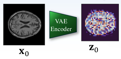
- A pre-trained variational auto-encoder \(V_{E,\phi}\) is fine-tuned on the dataset and then frozen for the rest of the process
- Each input image \(x^{(i)}\) are mapped to its latent space representation \(z^{(i)} = V_{E,\phi}\left(x^{(i)}\right)\), where \(z^{(i)} \in \mathbb{R}^{H' \times W' \times C'}\)
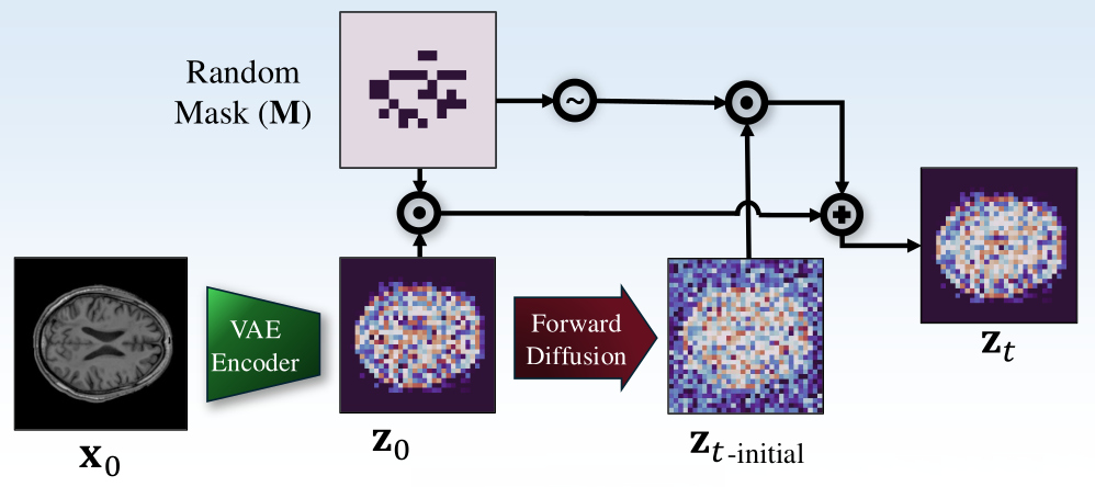
Random masking
- The latent features of a normal input sample \(z_0\) are spatially partitioned into non-overlapping patches using a random mask \(M \in [0,1]^{H' \times W'}\)
- This random mask simulates regions with abnormalities
Forward process
- The forward diffusion process gradually applies noise to the masked patches of sample \(z_0\) for \(t\) time steps to generate samples \(z_t\) with \(t \in [1, T]\)
\(z_t = \left( \sqrt{\bar{\alpha_t}} \, z_0 + \sqrt{1-\bar{\alpha_t}} \, \epsilon_t \right) \odot M + z_0 \odot \left( 1 - M \right)\)
where \(\epsilon_t \sim \mathcal{N}(0,I)\), \(\alpha_t = 1 - \beta_t\) and \(\bar{\alpha_t} = \prod_{i=1}^{T} \alpha_i\)
Reverse process
- The reverse process aims to recover the original data \(z_0\) by gradually removing the noise
- Given the sample \(z_t\) at step \(t\) and mask \(M\) at spatial location \(k\), the reverse process can be modeled as:
\(p\left(z^k_{t-1} \mid z^k_t\right) = \begin{cases} \mathcal{N}\left( \mu_{\theta}(z^k_t,t), \, \beta_t \mathbf{I} \right), &\textit{if } M^k=1 \\ z^k_t, & \textit{otherwise} \end{cases}\)
\(\mu_{\theta}(z_t,t)\) is a trainable function, which can be reparameterized as a predicted noise \(\epsilon\) or a predicted clean image \(z_0\)
-
Due to the incorporated random masking strategy, the predicted clean image formulation is chosen:
\(\mu_{\theta}(z_t,t) = \frac{\sqrt{\bar{\alpha}_{t-1}} \, \beta_t}{1-\bar{\alpha}_t} \, \color{red}{f_{\theta,z_0}(z_t,t)} + \frac{\sqrt{\alpha_t}\,(1-\bar{\alpha}_{t-1})}{1-\bar{\alpha}_t} \, z_t\)
where \(f_{\theta,z_0}(z_t,t)\) is a trainable function that predicts \(\hat{z}_0\) at time \(t\), given \(z_t\). - The following scheme is applied only to the masked region:
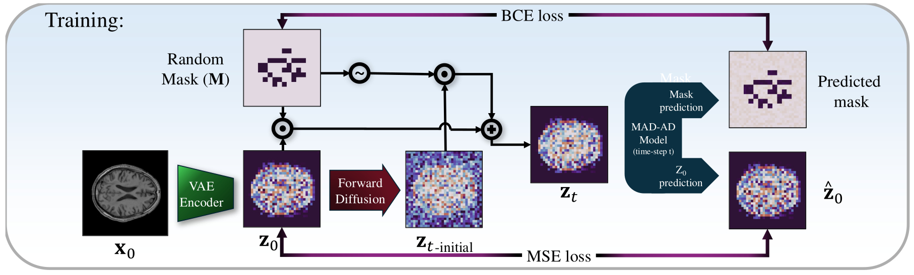
- \(f_{\theta,z_0}\) is a neural network that is trained using a simple mean-square error loss between \(z_0\) and the predicted image without any noise:
Mask prediction
- The location of the anomalous regions needs to be estimated during inference
- An additional head \(f_{\theta,M}\) is added to the diffusion model to predict the mask used in the forward diffusion process
-
The final loss function is given as: \(\displaystyle \min_{\theta} \; \mathbb{E}_{z_0 \sim q(z_0),\, \epsilon,\, t} \left[ \left\| z_0 - f_{\theta, z_0}(z_t, t) \right\|_2^2\right] + \lambda \, \mathcal{L}_{\mathrm{BCE}}\!\left(M, f_{\theta, M}(z_t, t)\right)\)
where \(\lambda\) is a hyper-parameter that balances the contributions of the two terms
Inference
Recovering normal images
- Let \(\{ x'^{(i)} \}_{i=1}^N\) denote the test set at inference time, which consists of samples with potential anomalies
- These images are first map into the latent space using \(V_{E,\phi}\)
The latent space of an anomalous image is treated as step \(T\) of a masked forward diffusion process applied on its normal counterpart, i.e., \(z'_T = V_{E,\phi}(x'_T)\)
-
By predicting the mask that corresponds to the anomaly location and the reconstructed \(\hat{z}'_0\) at each time-step \(t\), using the expression of \(p(z^k_{t-1} \mid z^k_t)\), it is possible to progressively correct the anomaly regions and obtain the normal counterpart \((z'_T \rightarrow z'_0)\) while preserving fine details of the normal regions
- One drawback of sampling with DDPM is that it requires many reverse sampling steps to obtain the normal version
- A DDIM framework is used instead to make the reverse process more deterministic and require fewer sampling steps
- The reverse process of DDIM is modified for the MAD-AD model as:
\(\begin{aligned} \tilde{z}'_{t-1} &= \underbrace{B\!\left(\color{red}{f_{\theta,M}(z'_t)}\right)}_{\text{predicted mask}} \Big( \sqrt{\bar{\alpha}_{t-1}}\, \underbrace{\color{red}{f_{\theta,z_0}(z'_t)}}_{\text{predicted } \hat{z}'_0} + \underbrace{\sqrt{1 - \bar{\alpha}_{t-1}}\, \color{red}{\hat{\epsilon}_t(z'_t)}}_{\text{direction pointing to } z'_t} + \sigma_t \epsilon'_t \Big) \\ &\quad + \left( 1 - B\!\left(\color{red}{f_{\theta,M}(z'_t)}\right) \right) z'_t \end{aligned}\)
where \(\hat{\epsilon}_t(z'_t) = \frac{z'_t - \sqrt{\bar{\alpha}_t}\,\color{red}{f_{\theta,z_0}}(z'_t)} {\sqrt{1-\bar{\alpha}_t}}\)
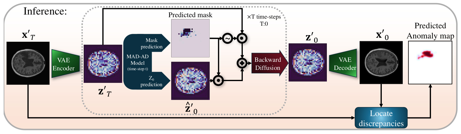
Anomaly localization
- The discrepancy between the input image and its reconstructed normal counterpart is used to localize anomalies
- Using the normal latent embedding \(\hat{z}'_0\), the normal sample is reconstructed in the image-space as: \(\hat{x}'_0 = V_{D,\phi}(\hat{z}'_0)\), where \(V_{D,\phi}\) is the pre-trained VAE decoder
- The predicted anomaly map is then given by
\(a = G * \min \left( \left\| \hat{x}'_0 - x'_0\right\|_2^2, \gamma \right) / \gamma\)
where \(G\) is a Gaussian kernel to smooth the predicted mask, \(∗\) is the convolution operator, and \(\gamma\) is a threshold designed to prevent assigning excessive weight to patches with significant deviations
Experiments
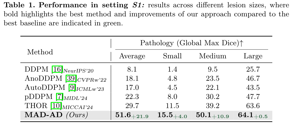
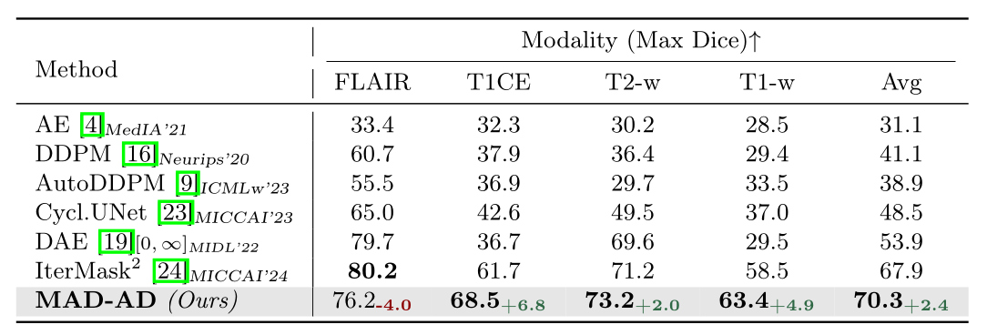
- The Maximum Dice score, which reports the highest value obtained for thresholds ranging from 0 to 1, is used to evaluate the performance of the anomaly detection model.
- A pre-trained VAE with perceptual loss and patch-based adversarial objective is used to project the data into a latent space, reducing the spatial dimension by a factor of 8
- The diffusion model corresponds to a standard UNet with attention
- The number of training and inference time-step (\(T\)) is set to 10
- To form the random mask at each iteration, the masking ratio is drawn from a uniform distribution \(U [0, 0.4]\), and the patch sizes of the mask along the \(X\) and \(Y\) axes are sampled independently from the following set: \(\{1, 2, 4, 8\}\)
- The random mask is then multiplied by the brain mask to prevent noise in non-brain
- The model was trained for 300 epochs using a batch size of \(96\) and AdamW optimizer with a learning rate of \(5 × 10^{−4}\)
Results
Setting-1 (S1)
- Training is performed on the middle slices of
IXI dataset, whereas only middle slices ofATLAS 2.0are used for testing
Setting-2 (S2)
BRATS’21 datasetis used. Normal slices are used for training, while the abnormal slice with the largest pathology is employed for inference.
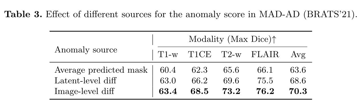
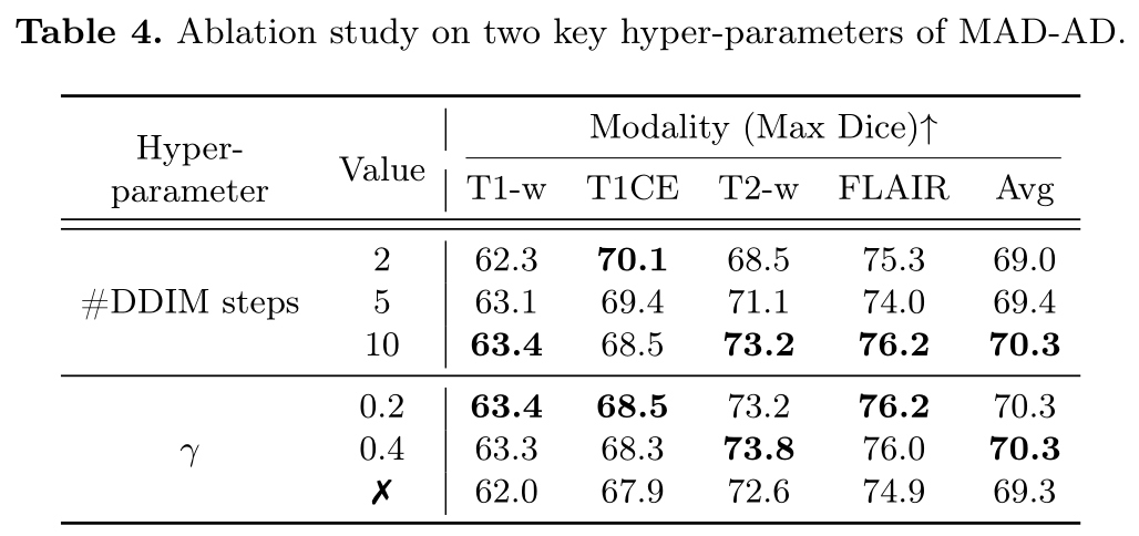
Ablation study
- Comparison of different strategies to form the anomaly map: pixel-level discrepancies \((x'_0,x'_T)\), latent-space discrepancies \((z'_0,z'_T)\), and the average of the predicted mask at reverse diffusion steps \(\frac{1}{T}\sum_{t=1}^T f_{\theta,M}(z'_t)\)
- Evaluation of the influence of key hyper-parameters on the performance of the proposed method
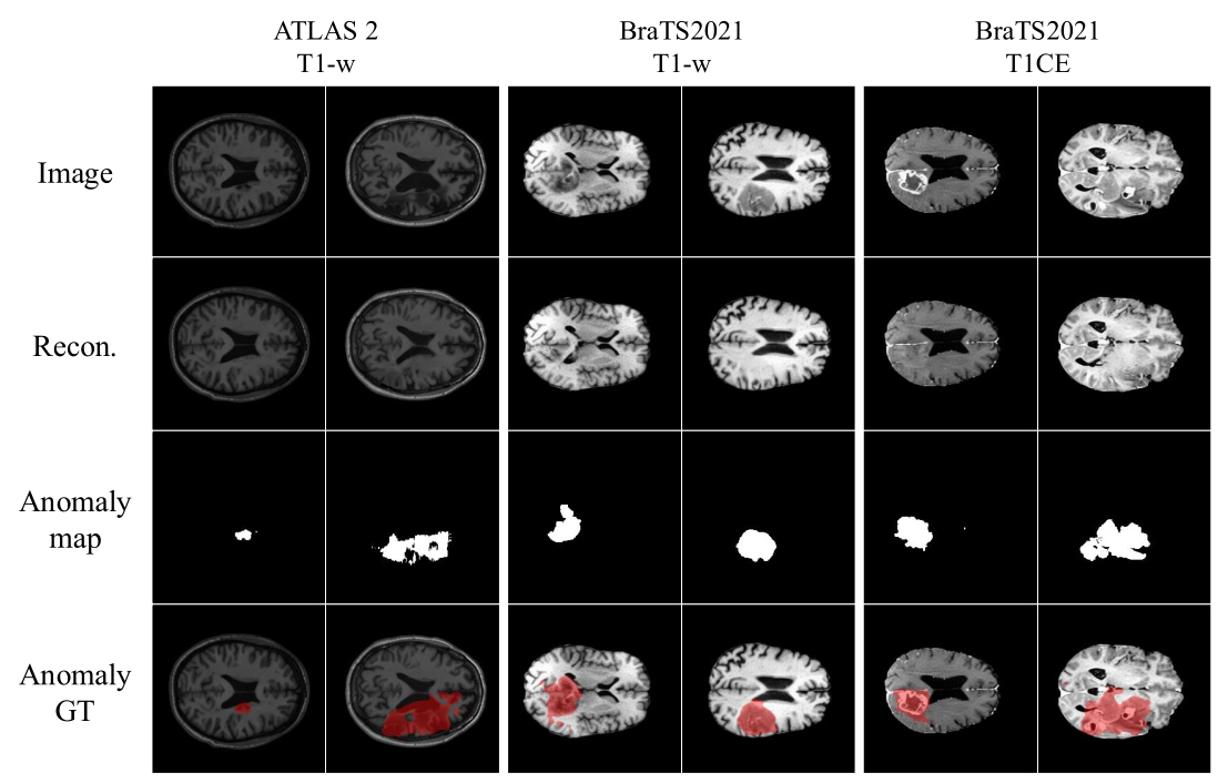
Qualitative results
Conclusions
- This paper presents an unsupervised anomaly detection
- The originality of the method is to introduce a unified formalism for forward and reverse diffusion processes applied consistently during training and inference
- The method beats state-of-the-art methods on two different settings involving three different datasets
Reference
-
Cosmin I. Bercea, Benedikt Wiestler, Daniel Rueckert, and Julia A. Schnabel. Diffusion Models with Implicit Guidance for Medical Anomaly Detection., MICCAI 2024 ↩