Brain Latent Progression: Individual-based Spatiotemporal Disease Progression on 3D Brain MRIs via Latent Diffusion
Highlights
- The authors propose Brain Latent Progression (BrLP), a novel spatiotemporal model designed to predict individual-level disease temporal progression in 3D brain MRIs.
- The framework addresses the need for individualization by explicitly integrating subject metadata and an auxiliary model to incorporate prior knowledge of disease dynamics.
- It introduces Latent Average Stabilization (LAS), an algorithm that enforces spatiotemporal consistency at inference and allows deriving a measure of prediction uncertainty.
- Link to the code here
Motivations
- Neurodegenerative diseases represent a major healthcare crisis, causing irreversible cognitive decline and requiring proactive strategies like early intervention and precision medicine.
- These diseases are notoriously complex and predicting their evolution in 3D brain MRIs faces four critical challenges that this paper tries to solve:
- Individualization: Accurately incorporating patient-specific clinical and demographic metadata.
- Longitudinal Data: Effectively exploiting a patient’s historical scans to understand their unique progression rate.
- Spatiotemporal Consistency: Ensuring the predicted future scans display a smooth, biologically plausible evolution without irregular artifacts.
- Memory Demand: Overcoming the massive computational resources required to process full 3D medical volumes.
Population-based vs. Individual-based Models
To understand the authors’ architectural choices, it is crucial to grasp the difference between the two main paradigms in disease progression modeling and their direct implications.
1. Population-based Models
- These models estimate an “average” disease trajectory based on a large population of affected subjects. Instead of using a patient’s real chronological age, they map everyone onto a shared “disease timeline” to account for different onset times and progression speeds. Predictions are made by adjusting this average trajectory to fit a specific patient.
- They provide highly interpretable insights into the general dynamics of a disease.
- Because they force individual patients onto an adjusted average path, which often fails to capture individual disease trajectories. Brain structures and disease patterns vary too widely between patients to be reduced to a simple variation of a population average.
2. Individual-based Models
- These models operate strictly at the individual level. They aim to predict how a specific subject’s high-dimensional data (like a full 3D scan) will change over a specified period. They use the patient’s actual chronological age as the timeline.
- They offer massive flexibility to handle unique, complex, and highly heterogeneous structural changes.
- This flexibility comes at a cost: it reduces the interpretability of the global, underlying disease dynamics compared to population models.
The choice is directly driven by the complexity of the disease. Since structural neurodegeneration in AD manifests very unevenly across different brain regions and patients, an “average” population trajectory would fail to capture the personalized nuances of the disease. An individual-based generative model is therefore necessary to synthesize these highly personalized, complex morphological changes.
Methodology
To effectively generate future MRIs, the authors propose a pipeline comprising four main components: an LDM, a ControlNet, an auxiliary model, and the LAS algorithm.
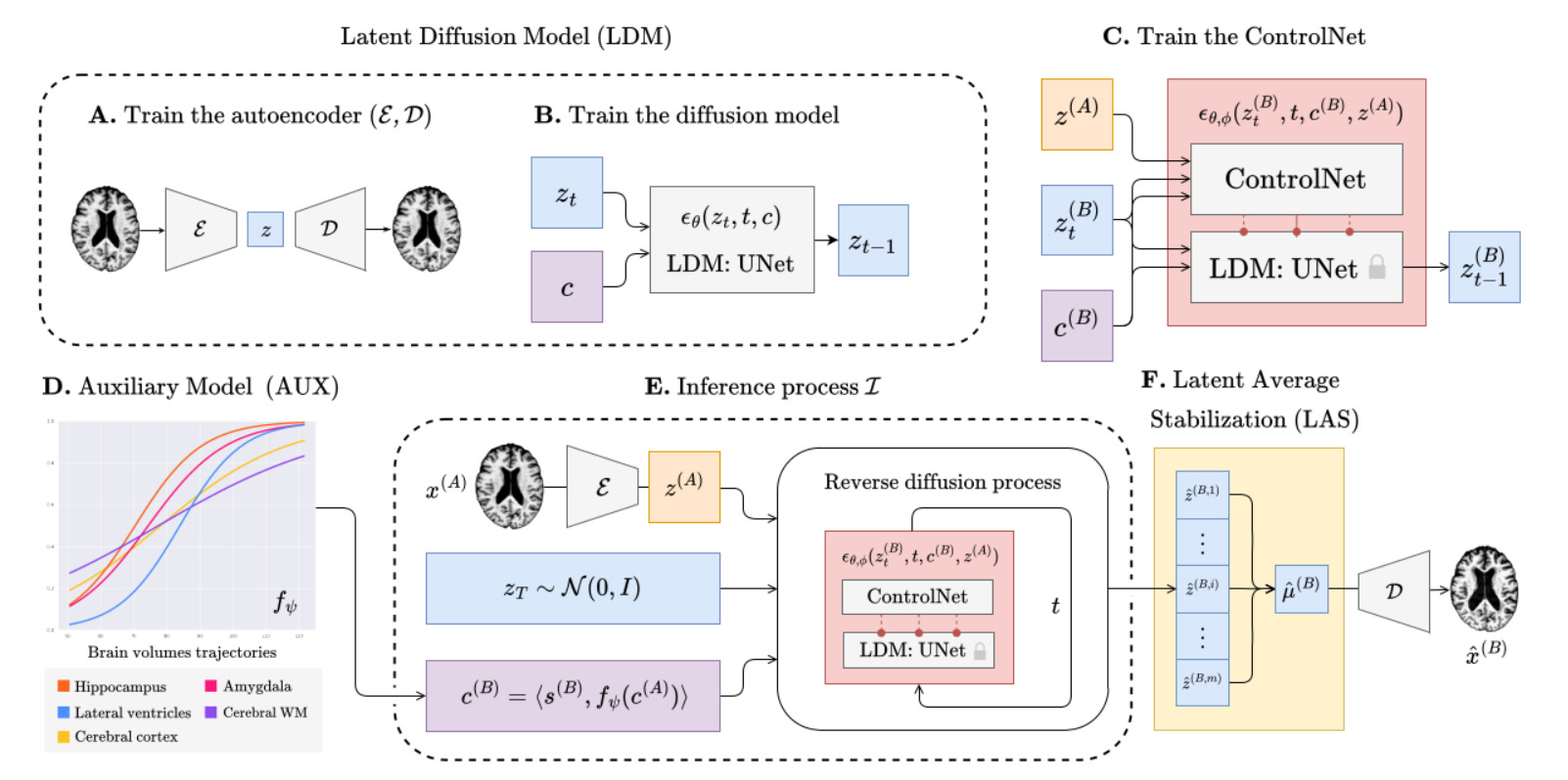
1. Latent Diffusion Model (LDM)
- Instead of applying diffusion in the high-dimensional pixel space, the authors train a variational autoencoder consisting of an encoder \(\mathcal{E}\) and a decoder \(\mathcal{D}\). The encoder compresses the 3D MRI \(x\) into a smaller latent space: \(z = \mathcal{E}(x)\).
- To guide the generation process so the output matches a specific patient’s profile, the model uses a combined set of conditioning variables, denoted as \(c=\langle s, v \rangle\). This vector concatenates two types of information:
- Subject-specific metadata: Age, sex, and cognitive status noted \(s\).
- Progression-related metrics: Volumes of specific brain regions strictly linked to Alzheimer’s Disease progression (hippocampus, cerebral cortex, amygdala, cerebral white matter, and lateral ventricles) noted \(v\).
- A conditional UNet is trained to estimate and remove the noise \(\epsilon_\theta(z_{t},t,c)\) added during the diffusion process in this latent space. The covariates \(c\) are injected into this UNet via a cross-attention mechanism.
2. Structural Conditioning via ControlNet
An LDM guided only by covariates \(c\) might generate a generic brain that matches the volumes but doesn’t look like the specific patient. It also cannot be conditionned on individual anatomical structures.
- To solve this, the authors use a ControlNet trained in conjunction with the LDM [^1].
- The ControlNet is specifically trained using latent representations from pairs of MRIs of the same patient taken at two different ages, \(A\) and \(B\) (with \(A < B\)). The latent representation of the patient’s baseline MRI, denoted \(z^{(A)}\), is used as an additional spatial condition to encompass the target brain’s structure during the generation process
- This forces the generative process to preserve the unique anatomical identity and structure of the patient’s brain across time.
3. Prior Knowledge via Auxiliary Model
To predict a future MRI at age \(B\), the model needs to know the future covariates \(v^{B}\) (the volumes of the AD-related regions). Learning the evolution of AD-related regions only from an MRI database is notoriously hard and gives little control over what is going on, even with a large deep-learning spatiotemporal model such as the ControlNet.
- The authors bypass this black-box limitation by using a dedicated auxiliary model \(f_{\psi}\) to predict how the volumes of AD-related regions will evolve.
- If only one baseline scan is available, a linear regression model that minimizes the Huber loss predicts the future volumes.
- If longitudinal data (past visits) is available, a Disease Course Mapping (DCM) [^2] algorithm is fitted to the patient’s history to predict a highly personalized volumetric trajectory.
4. Latent Average Stabilization
Because the inference process starts from random Gaussian noise \(z_T\) each time, running the process multiple times can yield slightly varying results, manifesting as irregular patterns or jittery transitions over multiple timesteps predictions.
To enforce strict spatiotemporal consistency, the authors propose the LAS algorithm, based on the assumption the predictions \(\hat{z}^{(B)}=\mathcal{I}(z_{T},x^{(A)},c^{(A)})\) deviate from a theoretical mean \(\mu^{(B)}\).
It consists of running the full inference process \(m\) times and computing the expected value of the latent representations before the final decoding step:
\[\mu^{(B)} \approx \frac{1}{m} \sum_{i=1}^{m} \mathcal{I}(z_{T, i}, x^{(A)}, c^{(A)})\]The final predicted scan is then decoded as \(\hat{x}^{(B)} = \mathcal{D}(\mu^{(B)})\).
The authors also use the standard deviation of these \(m\) predictions as a uncertainty measure:
\[\sigma^{(B)} \approx \sqrt{\frac{\sum_{i=1}^{m}(z_{i}^{(B)}-\mu^{(B)})^2}{m}}\]The Inference Process
The inference process is the most critical part of the framework. It brings all the aforementioned blocks together to predict a subject’s future brain MRI at a target age \(B\), starting from a baseline MRI \(x^{(A)}\) at age \(A\).
The process follows these exact steps:
- Volume Prediction: The auxiliary model predicts the future progression-related volumes \(\hat{v}^{(B)}\) at the target age \(B\).
- Covariate Formation: These predicted volumes are concatenated with the future metadata to form the target covariates \(c^{(B)} = \langle s^{(B)}, \hat{v}^{(B)} \rangle\).
- Encoding: The baseline MRI is encoded into the latent space to get \(z^{(A)} = \mathcal{E}(x^{(A)})\).
- Noise Sampling: Gaussian noise \(z_T \sim \mathcal{N}(0, I)\) is sampled.
- Reverse Diffusion: The unified LDM and ControlNet model predicts the noise to iteratively reverse the diffusion steps from \(T\) down to \(0\), explicitly conditioned on both the future covariates \(c^{(B)}\) and the baseline anatomy \(z^{(A)}\).
- Latent Average Stabilization: They repeat the inference process \(m\) times and compute the average result \(\mu^{(B)}\)
- Decoding: The final denoised latent \(\mu^{(B)}\) is passed through the decoder \(\mathcal{D}\) to generate the predicted 3D MRI \(\hat{x}^{(B)}\).
Experiments & Results
1. Datasets and Experimental Settings
- Datasets: The model was trained internally on 11,730 T1w MRIs from 2,805 subjects (combining ADNI, OASIS-3, and AIBL). To prove robust generalization, it was tested on an external dataset (NACC) comprising 2,257 MRIs from 962 subjects.
- Baselines: BrLP was compared against existing generative approaches: DaniNet, CounterSynth, and Latent-SADM.
- Settings: The models were evaluated in two scenarios: Single-image (predicting future progression from only one baseline scan) and Sequence-aware (using multiple past visits to predict the future).
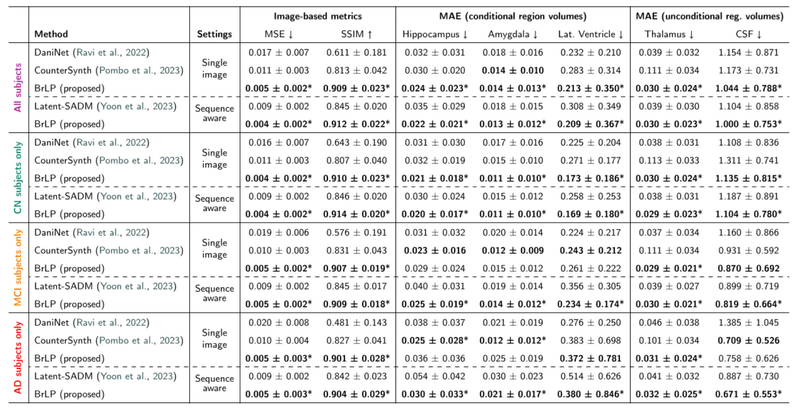
- Evaluation Metrics: They use MSE and SSIM to evaluate the similarity between scans and compute the MAE between the volumes of the generated scan and actual follow-up scan to assess the model’s accuracy in tracking disease progression. Some regions (Cerebrospinal Fluid (CSF) and thalamus) are excluded from covariates \(v\) to evaluate the model predictions on unconditionned regions.
2. Ablation Study: The Impact of AUX and LAS
The authors isolated the contributions of the Auxiliary model (AUX) and the Latent Average Stabilization (LAS) algorithm:
AUX
- Introducing the AUX model alone led to a 16% reduction in volumetric errors.
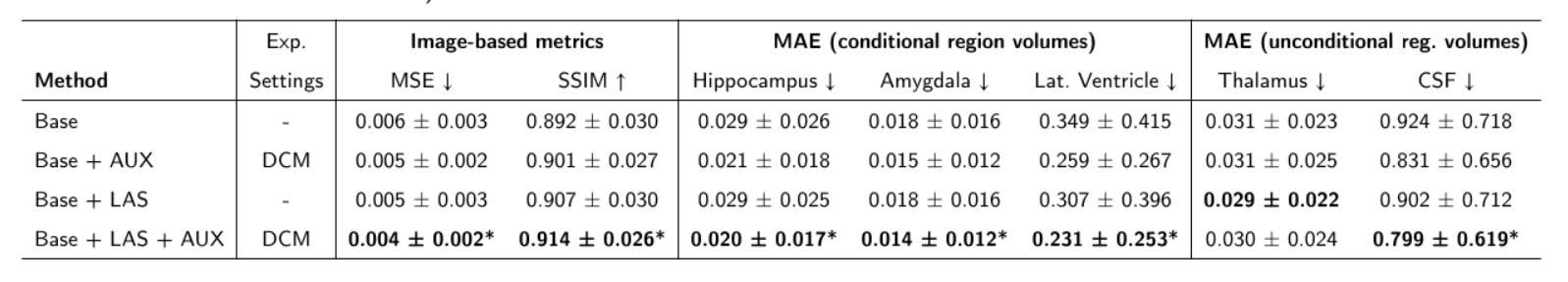
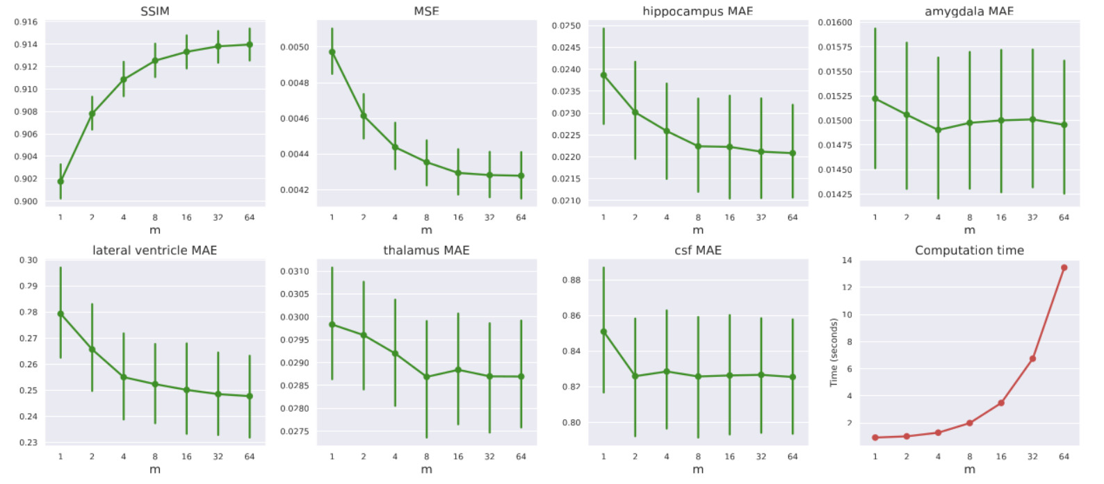
LAS
- Tuning LAS (\(m\)): Increasing the LAS hyperparameter \(m\) from 2 to 64 steadily improved performance: MSE decreased by 7%, volumetric errors reduced by 3%, and SSIM improved by 0.68%. However, this introduces a direct trade-off with computation time. From now on, all the presented experiments are conducted with \(m=64\)
- The LAS algorithm contributed an additional 4% reduction. Combined, they yield a 21% reduction in volumetric errors.
- Quantifying Uncertainty: The standard deviation across the \(m\) predictions acts as a reliable clinical uncertainty score. The authors proved statistically that higher model uncertainty correlates directly with higher MSE and lower SSIM, meaning the model “knows” when it is likely making a less accurate prediction.
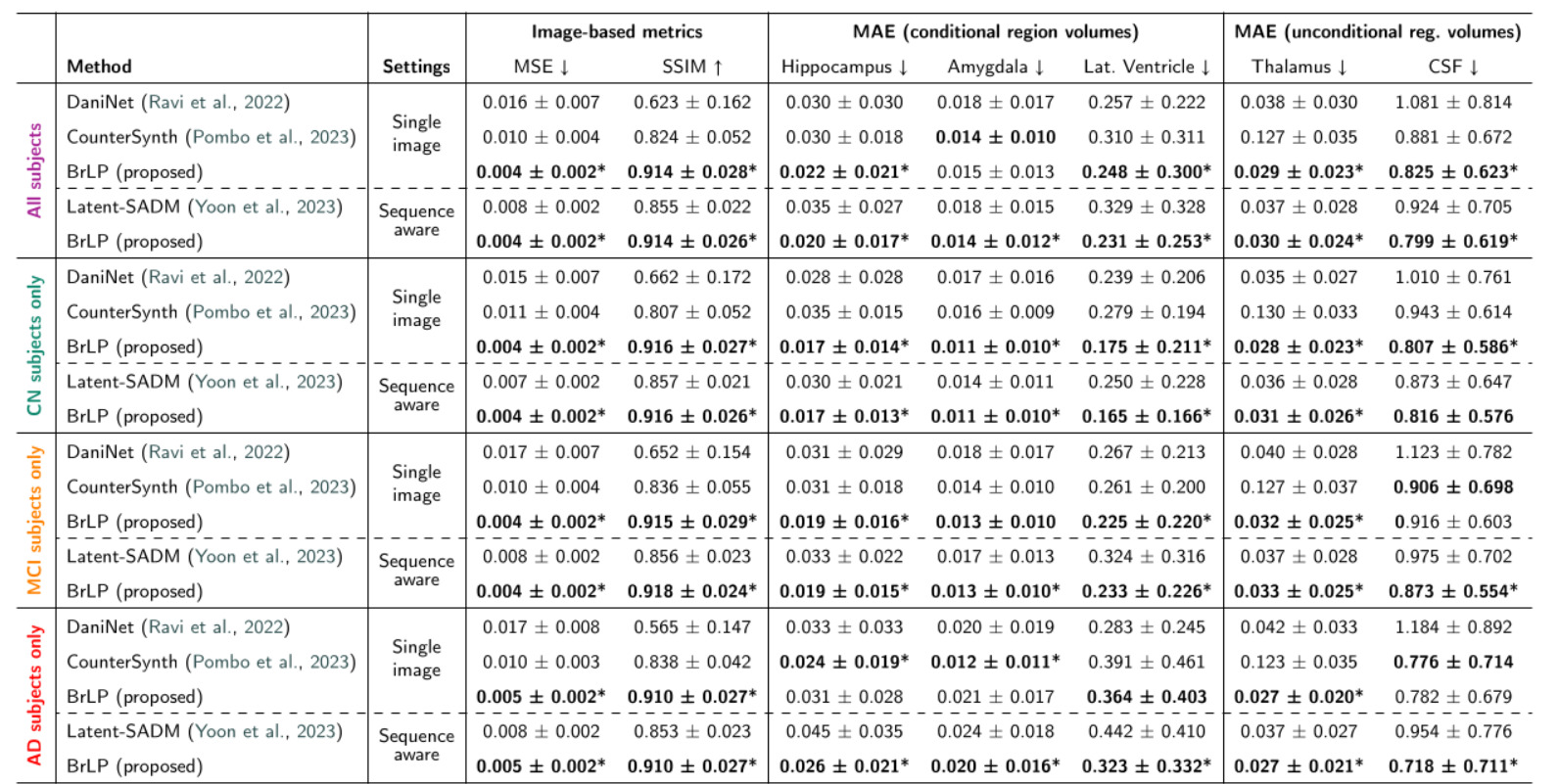
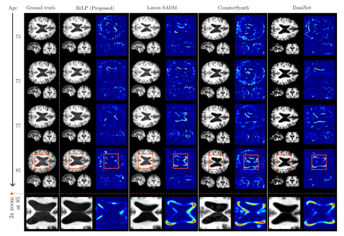
3. State-of-the-Art Comparisons
BrLP vastly outperformed all baselines on both image-based and volumetric metrics across both test sets:
- Internal Test Set: BrLP achieved an average MSE reduction of 61.67% and an SSIM increase of 21.51%. For tracking AD-related volumetric changes, it improved accuracy by 18.84% over DaniNet, 24.61% over CounterSynth, and 25.46% over Latent-SADM.
- External Test Set: The model proved its out-of-distribution robustness by maintaining its lead, showing a 60.23% MSE reduction and a 22.84% SSIM increase over baselines.
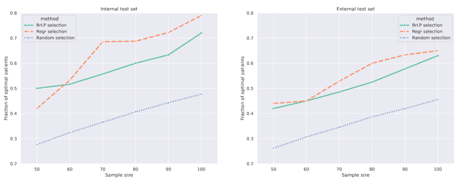
4. Downstream Application: Patient Selection for Clinical Trials
One major application is avoiding Type II errors in clinical trials. These errors occur when a study fails to prove a drug’s efficacy because the selected patients progress too slowly to show a measurable effect within the trial’s timeframe.
- To identify “fast progressors”, the authors focus on hippocampal atrophy. BrLP generates the patient’s predicted 3D MRI two years into the future, from which the predicted hippocampal volume is extracted. The top \(S\) candidates with the largest predicted volume reductions are then selected for the trial.
- BrLP was compared to a standard linear regression model (a Huber Regressor robust to outliers, the same one used to estimate volume progression in the Auxiliary model) that directly predicts future volumes from baseline tabular data without generating any image.
- While the highly-specialized regression model selected slightly more optimal patients on the internal dataset, BrLP showed superior robustness. The regression model suffered a 6.82% performance drop on the external dataset, whereas BrLP only dropped by 5.17%.
Conclusions
- BrLP establishes a new state-of-the-art for individual-based 3D brain MRI progression using Latent Diffusion.
- By dividing the problem by using an auxiliary model for trajectory prediction and a conditioned diffusion model for anatomical generation they ensure high biological fidelity.
- The Latent Average Stabilization (LAS) algorithm is a highly effective, simple mechanism to force temporal smoothness and extract prediction uncertainty.