Unsupervised Blind Source Separation with Variational Auto-Encoders
Blind Source Separation (BSS)
Problem definition
Given an observed mixed signal \(x\) made from the sum of \(M\) sources \(s_m\) and noise \(\epsilon\) such that:
\[x = \sum_{m=1}^{M} s_m + \epsilon,\]we want to find source estimates \(\hat{s}_m\) and the number of underlying sources \(M.\) This is a highly undetermined problem.
Examples: cocktail party problem (audio), disentangle multiple objects superimposed on a single picture (image), recover blood signal from an echography acquisition (ultrasound signal), etc.
Methods to solve this problem
Classic methods include:
- Independent Component Analysis (ICA),
- Principal Component Analysis (PCA),
- Non-negative Matrix Factorisation (NMF),
- etc.
The inconvenients of these methods is that they require iterative procedures that can be time consuming, may need to manually set some parameters or to assume properties about the sources.
Deep learning methods are also used in supervised or semi-supervised settings such as:
- Supervised and semi-supervised VAE,
- Supervised VAE-NMF hybrid method,
- Deep clustering,
- Mixtures of generative latent optimization (GLO),
- Mixture invariant training (MixIT),
- etc.
The problem with these methods is the need of a training dataset with pairs of mixed signals and the unmixed sources, and/or the need to know a priori the number \(M\) of sources to unmix.
In this work, the authors propose a fully unsupervised VAE for BSS.
Proposed method: Variational Auto-Encoder (VAE)
(For more details, look at the tutorial on VAE)
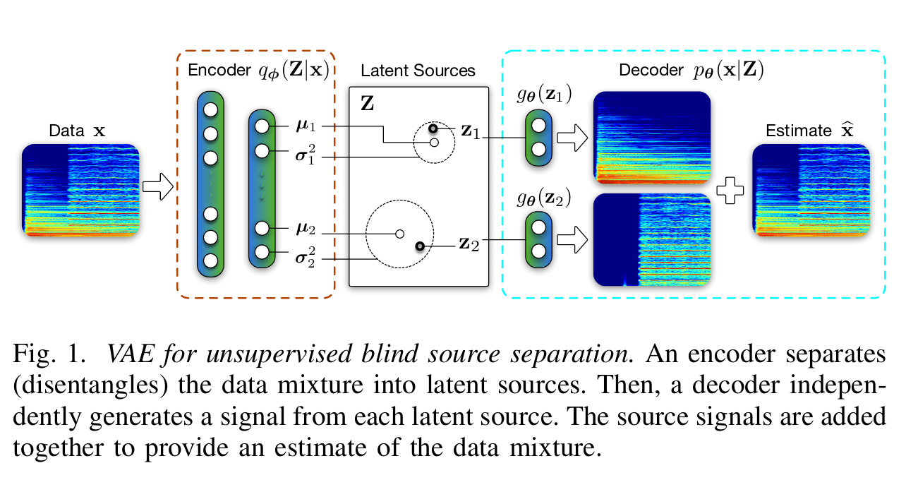
Decoder
The decoder is given by the function \(g_\theta\) such that
\[\hat{s}_k = g_\theta(z_k)\]where \(\hat{s}_k\) is an estimated source and \(z_k\) a latent source. Defining \(z=\{z_k\}_{k=1}^K\) the concatenation of all latent sources, the estimate of the mixed data is given by
\[\hat{x} = \sum_{k=1}^K \hat{s}_k = \sum_{k=1}^K g_\theta(z_k).\]The error \(\epsilon\) is assumed to follow a zero-mean Laplace distribution with scale \(b = \sqrt{0.5}\) for unit-variance. The likelihood of signal \(x\) given \(z\) is then defined as:
\[p_\theta(x|z) = \prod_{i=1}^n p(x_i|\hat{x_i}) = \prod_{i=1}^n \text{Lap}(x_i|\hat{x_i},b) = \prod_{i=1}^n \frac{1}{2b} \text{exp}\left(-\frac{|x_i - \hat{x}_i|}{b}\right),\]where \(n\) is the dimension of \(x.\) The authors argue that considering a Laplace likelihood instead of a Gaussian one penalizes deviations around the mean and thus prevents blurry reconstructions.
Encoder
The prior \(p(z)\) enforces each source element to follow a zero-mean, unit variance Gaussian distribution:
\[p(z) = \prod_{k=1}^K p(z_k) = \prod_{k=1}^K N(z_k | 0, I).\]Given the signal \(x,\) the posterior \(q_\phi(z|x)\) is defined such that the elements of \(z\) are independent and Gaussian distributed,
\[q_\phi(z|x) = N(z|\mu_\phi(x), \sigma^2_\phi(x) I).\]Loss function
Using variational inference, they maximize the lower bound:
\[L(\theta, \phi; x) = ln(p_\theta(x|z)) - D_{KL}(q_\phi(z|x) || p(z))\]The loss is then defined as:
\[\text{loss} = |x - \hat{x}| - \beta * D_{KL}(N(\mu_\phi(x), \sigma^2_\phi(x)), N(0,I))\]The \(\beta\text{-VAE}\) formulation is used to avoid posterior collapse early in training, with \(\beta = 0.5.\)
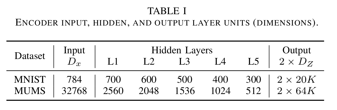
Experimental settings
- The encoder and decoder each had 5 fully connected feed-forward layers.
-
The true number of sources \(M\) is always of 2, and the number of assumed sources \(K\) is set to 2, 3 and 4, to see if the performance degrades when \(M \neq K.\)
-
The inferred sources \(\hat{s}_k\) are converted to mask-based estimates \(\check{s}_k\) (VAEM) to constrain the sum of estimated sources to exactly match the data:
-
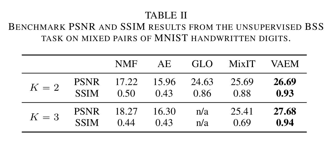
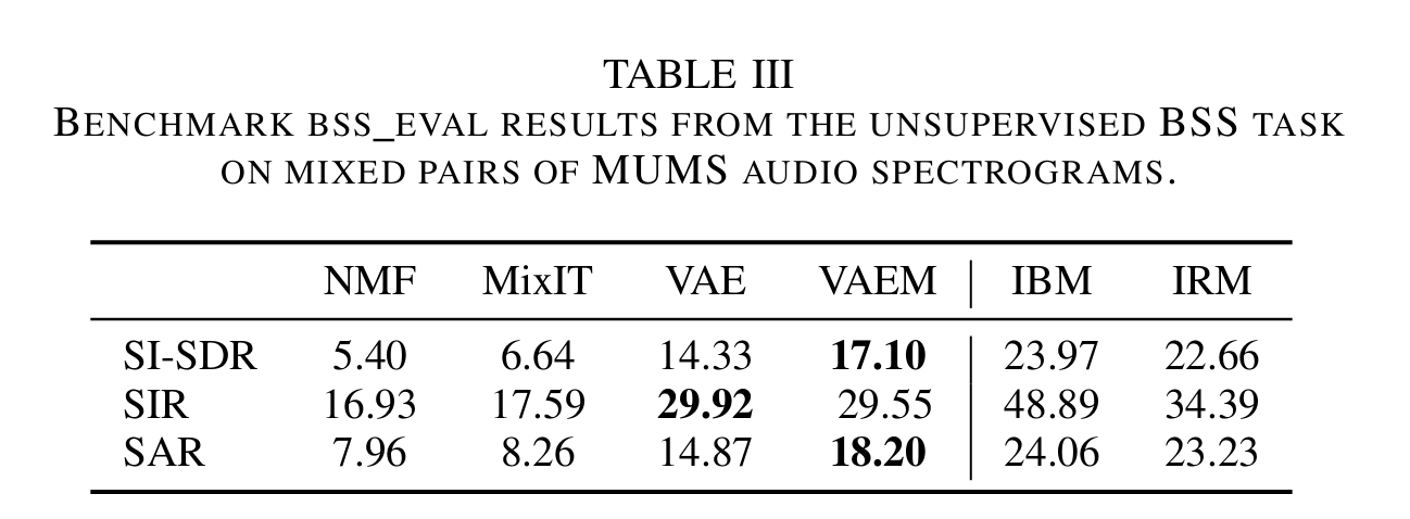
Baseline methods include: a classic method (NMF), an auto-encoder (AE), a semi-supervised method (GLO) and an unsupervised method (MixIT). Ideal binary masks (IBM) and ideal ratio masks (IRM) provide upper-bound performances.
-
Their code is available here.
Results
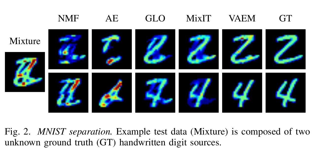
- Results on MNIST images.
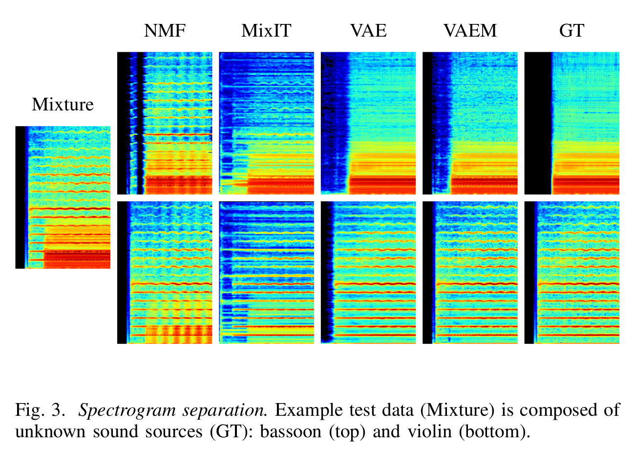
- Results on spectrograms. Metrics include: scale-invariant signalto-distortion ratio (SI-SDR), signal-to-interference ratio (SIR), and signal-to-artifact ratio (SAR).
Conclusions
- They proposed an unsupervised solution to BSS.
- The model achieved good results on two different application domains.
- Sources are generated using the same decoder, so the model is independent of the number of sources.
- Further experiments need to be made to test the robustness of the architecture in more complex settings.