The variational autoencoder paradigm demystified
Notes
- Here are links to four video that I used to create this tutorial: video1, video2, video3, video4.
- I was also strongly inspired by this excellent post.
Intuition
Autoencoder VS PCA
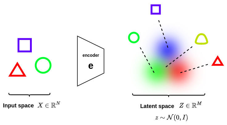
Let’s start with the basic representation of an autoencoder
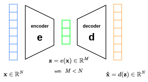
Autoencoders belong to the family of dimension reduction methods. This method takes as input a vector \(\mathbf{x} \in \mathbb{R}^N\) and outputs a closed vector \(\mathbf{\hat{x}} \in \mathbb{R}^N\) with the restriction of passing through a space with reduced dimensionality \(Z \in \mathbb{R}^M\). This is usually achieved through the minimization of the \(L_2\) norm function: \(\lVert \mathbf{x} - \mathbf{\hat{x}} \rVert^2\).
\(\mathbf{e}\) and \(\mathbf{d}\) are two different networks that model the (non linear) mappings from the input space \(X\) to the latent space \(Z\) in both directions.
Let us now consider the simple case where \(\mathbf{e}\) and \(\mathbf{d}\) correspond to two single-layer networks without any non-linearity. The corresponding autoencoder can be represented as follows:
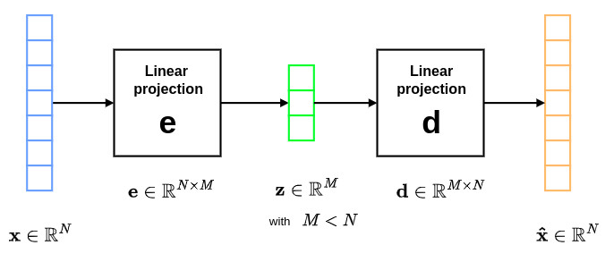
where \(\mathbf{e} \in \mathbb{R}^{N \times M}\) and \(\mathbf{d} \in \mathbb{R}^{M \times N}\) are two linear matrices. In the particular case where \(\mathbf{e} = \mathbf{U}^T\) and \(\mathbf{d} = \mathbf{U}\), the autoencoder expressions can be written as:
\[\mathbf{z} = \mathbf{U}^T\mathbf{x} \quad\quad \text{and} \quad\quad \mathbf{\hat{x}} = \mathbf{U}\mathbf{z}=\mathbf{U}\mathbf{U}^T\mathbf{x}\]This corresponds to the well know PCA (Principal Component Analysis) paradigm. A more formal proof can be found in this article.
Autoencoders can thus be seen as a generalization of the dimensionality reduction PCA formalism by evolving more complex operations defined through \(\mathbf{e}\) and \(\mathbf{d}\) networks.
Why get hurt with a probabilistic context?
VAEs can be considered as an extension of autoencoders with the introduction of regularization mechanisms (encoder side) to ensure that the generated latent space has good properties allowing the generative process (decoder side). The regularity that is expected from the latent space in order to make generative process possible can be expressed through two main properties:
- continuity: two close points in the latent space should give close contents when decoded.
- completeness: a point sampled from the latent space should give “meaningful” content once decoded.
These two aspects are optimized within VAEs thanks to a probabilistic framework.
Continuity
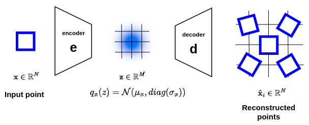
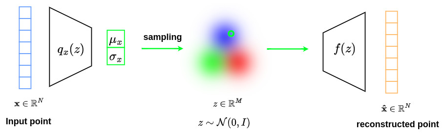
In order to introduce local regularization to structure the latent space, the encoding-decoding process is slightly modified: instead of encoding an input as a single point, we encode it as an axis-aligned Gaussian distribution \(q_x(z) = \mathcal{N}\left(\mu_x,diag\left(\sigma_x\right)\right)\) over the latent space. Thus, a point \(x\in \mathbb{R}^N\) at the input of the encoder will correspond to a Gaussian distribution \(q_x(z)\) at the output, as shown below:

This will ensure that the sampling of a local region in the latent space should produce results that are close.
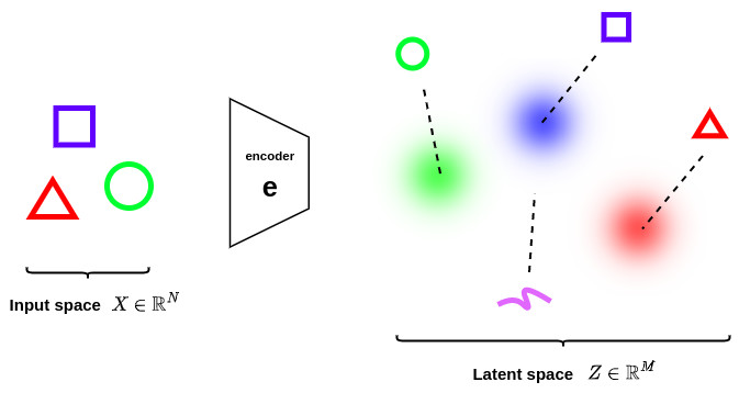
However, this property is not sufficient to guarantee continuity and completeness. Indeed encoder can either learn distributions with tiny variances (which would correspond to classical autoencoders) or return distributions with very different means (which would be far apart from each other in the latent space), as illustrated in the figure below.
Completeness
In order to avoid these effects the covariance matrix and the mean of the distributions returned by the encoder need to be also regularized. In practice, this new regularization is done by enforcing distributions to be close to a standard normal distribution \(\mathcal{N}\left(0,I\right)\). This way, the covariance matrices are required to be close to the identity, preventing punctual distributions, and the mean to be close to 0, preventing encoded distributions to be too far apart from each other, as illustrated in the figure below.
Thanks to this regularization strategy, we prevent the model to encode data far apart in the latent space and encourage as much as possible returned distributions to overlap, satisfying this way the expected continuity and completeness conditions!
Using the previous reasoning, the overall architecture of the VAE can be represented as follows.
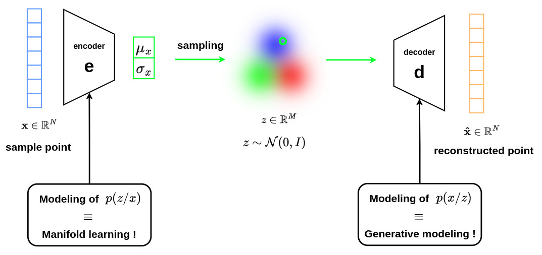
VAE thus offers two extremely interesting opportunities:
-
the mastery of the encoder allows to optimize the mapping operation \(p(z \vert x)\) to a latent space with reduced dimensionality for interpretation purposes. This corresponds to manifold learning paradigm.
-
the mastery of the decoder allows to optimize the mapping operation \(p(x \vert z)\) for the generation of data with a complex distribution. This corresponds to generative model framework.
In the rest of this tutorial, we will see how the VAE formalism allows to optimize these two tasks through the theory of variational inference.
Fondamental concepts
Information quantification
Information \(I\) can be quantified through the following expression:
\[I = -log(p(x))\]with \(x\) being an event and \(p(x)\) the probability of this event. Since \(0\leq p(x) \leq 1\), \(I\) is positive and tends to infinity when \(p(x)=0\).
From this equation, one can see that when the probability of an event is high (close to \(1\)), the corresponding information is low, which makes sense. For instance, the probability that the weather will be hot in France during summer is very high, so this sentence does not provide any useful information in a conversation
Please note that the information \(I\) comes with a unit. If the log is a natural logarithm, we call it a “nat” and if the log has a base 2, we call it a “bit”, just like the binary information stored in a computer. Think about it, if you randomly pick one such binary variable in a computer, its chance of being \(0\) or a \(1\) is \(50\%\). Thus, the information associated to the event of observing a \(0\) or a \(1\) in a binary computer variable is:
\[-log_2\left(\frac{1}{2}\right)=log_2(2)=1\]i.e., one bit.
Entropy
Entropy \(H\) corresponds to the average information of a process. Its expression can be naturally written as:
\[H = -\sum_{i=1}^{N}{p(x_i)\cdot log\left(p(x_i)\right)} \quad \quad \quad \text{or} \quad \quad \quad H = -\int{p(x)\cdot log\left(p(x)\right)}\,dx\]Since the information \(-log\left(p(x)\right)\) is always positive and that \(p(x)\) is also positive, then the entropy \(H\) is also positive!
Kullback-Liebler divergence
The Kullback-Liebler (KL) divergence allows to measure the distance between two distributions through the use of relative entropy concepts. Let’s define the following expressions:
\[H_{p} = -\int{p(x)\cdot log\left(p(x)\right)}\,dx\] \[H_{pq} = -\int{p(x)\cdot log\left(q(x)\right)}\,dx\]where \(H_{p}\) corresponds to the entropy relative to the distribution \(p(x)\) and \(H_{pq}\) the average information brought by \(g(x)\) but weighted by \(p(x)\). Note that one can prove that \(H_{pq}>H_{p}\) whever \(p\neq q\).
From these notations, the KL divergence \(D_{KL}\) can be expressed as:
\[D_{KL}\left(p \parallel q \right) = H_{pq} - H_{p}\] \[D_{KL}\left(p \parallel q \right) = -\int{p(x)\cdot log\left(q(x)\right)}\,dx + \int{p(x)\cdot log\left(p(x)\right)}\,dx\] \[D_{KL}\left(p \parallel q \right) = -\int{p(x)\cdot log\left(\frac{q(x)}{p(x)}\right)}\,dx\] \[D_{KL}\left(p \parallel q \right) = \int{p(x)\cdot log\left(\frac{p(x)}{q(x)}\right)}\,dx\]KL divergence allows to measure a distance between two distributions with the following properties:
- \(D_{KL}\) is always positive (because \(H_{pq}>H_{p}\)): \(\quad \quad D_{KL}\left(p \parallel q \right) \geq 0\)
- \(D_{KL}\) is not symmetric: \(\quad \quad D_{KL}\left(p \parallel q \right) \neq D_{KL}\left(q \parallel p \right)\)
Here is a graph to intuit the second relationship, i.e. \(D_{KL}\) is not symmetric.

Indeed, from the perspective of the purple distribution, the distance between points A and B appears to be high. However, from the perspective of the green distribution, the same distance appears to be moderate.
\(D_{KL}\) can thus be used to measure a distance between two distributions. Its is always positive and it is not symmetric.
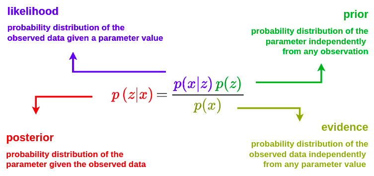
Bayes theorem
Let’s assume a model where data \(x\) are generated from a probability distribution depending on an unknown parameter \(z\). Let’s also assume that we have a prior knowledge about the parameter \(z\) that can be expressed as a probability distribution \(p\left(z\right)\). Then, when data \(x\) are observed, we can update the prior knowledge about this parameter using Bayes theorem as follows:
Variational inference
Key concept
In the VAE formalism, we first make the assumption that \(p(z)\) is a standard Gaussian distribution (to ensure completeness) and that \(p(x \vert z)\) is a Gaussian distribution whose mean is defined by a deterministic function \(f\) of the variable \(z\) and whose covariance matrix has the form of a positive constant \(c\) that multiplies the identity matrix \(I\). We will see that this last assumption allows to keep most of the information of the data structure in the reduced representations.
\[p(z) = \mathcal{N}(0,I)\] \[p(x \vert z) = \mathcal{N}(f(z),cI)\]The key concept around VAE is that we will try to optimize the computation of the non-linear mapping \(p(z \vert x)\). Indeed, it can be demonstrated that the computation of \(p(z \vert x)\) is often complicated and requires the use of approximation techniques such as variational inference.
In statistics, variational inference is a technique to approximate complex distributions. The idea is to set a parametrised family of distributions, usuall the family of Gaussians whose parameters are the mean and the covariance, and to look for the best approximation of the target distribution among this family. The best element in the family is one that minimise a given approximation error measurement, most of the time the KL divergence between approximation and target.
In the VAE formalism, \(p(z \vert x)\) is modeled by an axis-aligned Gaussian distribution \(q_x(z)\) whose mean \(\mu_x\) and covariance \(\sigma_x\) are defined by two functions \(g(x)\) and \(h(x)\).
\[q_x(z) = \mathcal{N}\left(\mu_x,diag\left(\sigma_x\right)\right) = \mathcal{N}\left(g(x),diag\left(h(x)\right)\right)\]We thus have a family of candidates for variational inference and need to find the best approximation among this family by minimising the KL divergence between the approximation \(q_x(z)\) and the target \(p(z \vert x)\). In other words, we are looking for the optimal \(g^*\) and \(h^*\) such that:
\[\left(g^*,h^*\right) = \underset{(g,h)}{\arg\min} \,\,\, D_{KL}\left(q_x(z) \parallel p(z \vert x) \right)\]Let’s now reformulate the KL divergence expression.
\[D_{KL}\left(q_x(z) \parallel p(z \vert x) \right) = - \int{q_x(z) \cdot log\left(\frac{p(z \vert x)}{q_x(z)}\right) \,dz}\]By using the conditional probability relation:
\[p(z \vert x) = \frac{p(x,z)}{p(x)}\]where \(p(x,z)\) is the joint distribution of event \(x\) and \(z\), the above expression can be rewritten as:
\[D_{KL}\left(q_x(z) \parallel p(z \vert x) \right) = - \int{q_x(z) \cdot log\left(\frac{p(x,z)}{p(x) \cdot q_x(z)}\right) \,dz}\] \[D_{KL}\left(q_x(z) \parallel p(z \vert x) \right) = - \int{q_x(z) \cdot \left[ log\left(\frac{p(x,z)}{q_x(z)}\right) + log\left(\frac{1}{p(x)}\right) \right] \,dz}\] \[D_{KL}\left(q_x(z) \parallel p(z \vert x) \right) = - \int{q_x(z) \cdot log\left(\frac{p(x,z)}{q_x(z)}\right) \,dz} \,+\, log\left(p(x)\right) \cdot \underbrace{\int{q_x(z)\,dz}}_{=1}\] \[D_{KL}\left(q_x(z) \parallel p(z \vert x) \right) \,+\, \mathcal{L} \,=\, log\left(p(x)\right)\]where \(\mathcal{L}\) is defined as the Evidence Lower BOund (ELBO) whose expression is given by:
\[\mathcal{L} = \int{q_x(z) \cdot log\left(\frac{p(x,z)}{q_x(z)}\right) \,dz}\]
Evidence lower bound
Let’s take a closer look at the previous derived equation:
\[D_{KL}\left(q_x(z) \parallel p(z \vert x) \right) \,+\, \mathcal{L} \,=\, log\left(p(x)\right)\]The following observations can be made:
-
since \(0\leq p(x) \leq 1\), \(log\left(p(x)\right) \leq 0\)
-
since \(x\) is the observation, \(log\left(p(x)\right)\) is a fixed value
-
by definition \(D_{KL}\left(q_x(z) \parallel p(z \vert x) \right) \geq 0\)
-
since \(\mathcal{L} = -D_{KL}\left(q_x(z) \parallel p(x,z)\right)\), \(\mathcal{L} \leq 0\)
The previous expression can thus be rewritten as follows:
\[\underbrace{D_{KL}\left(q_x(z) \parallel p(z \vert x) \right)}_{\geq 0} \,+\, \underbrace{\mathcal{L}}_{\leq 0} \,=\, \underbrace{log\left(p(x)\right)}_{\leq 0 \,\, \text{and fixed}}\]At this point, it is important to remember that \(p(z \vert x)\) is the unknown and that the goal is to find the best \(q_x(z)\), i.e. the one that shall minimize \(D_{KL}\left(q_x(z) \parallel p(z \vert x) \right)\).
With the above observations, the following strategy can be implemented: by tweaking \(q_x(z)\), we can seek to maximize the ELBO \(\mathcal{L}\), which will imply the minimization of the KL divergence \(D_{KL}\left(q_x(z) \parallel p(z \vert x) \right)\), and thus to find a distribution \(q_x(z)\) that is close to \(p(z \vert x)\). The table below provides an illustration of such a strategy.
| \(\downarrow \, D_{KL}\) | \(\uparrow \, \mathcal{L}\) | \(log\left(p(x)\right)\) |
|---|---|---|
| 4 | -8 | -4 |
| 3 | -7 | -4 |
| 2 | -6 | -4 |
| 1 | -5 | -4 |
| 0 | -4 | -4 |
ELBO reformulation
The ELBO \(\mathcal{L}\) should be reformulated so to justify the loss involved in the VAE framework. The corresponding derivation is provided below.
\[\mathcal{L} = \int{q_x(z) \cdot log\left(\frac{p(x,z)}{q_x(z)}\right) \,dz}\]By using the conditional probability relation:
\[p(x \vert z) = \frac{p(x,z)}{p(z)}\]the above expression can be rewritten as:
\[\mathcal{L} = \int{q_x(z) \cdot log\left(\frac{p(x \vert z)\cdot p(z)}{q_x(z)}\right) \,dz}\] \[\mathcal{L} = \int{q_x(z) \cdot \left[ log\left(p(x \vert z)\right) + log\left(\frac{p(z)}{q_x(z)}\right) \right] \,dz}\] \[\mathcal{L} = \int{q_x(z) \cdot log\left(p(x \vert z)\right) \,dz} + \int{q_x(z) \cdot log\left(\frac{p(z)}{q_x(z)}\right) \,dz}\] \[\mathcal{L} = \mathbb{E}_{z\sim q_x} \left[log\left(p(x \vert z)\right)\right] - D_{KL}\left(q_x(z)\parallel p(z)\right)\]where \(\mathbb{E}_{z\sim q_x}\) is the mathematical expectation with respect to \(q_x(z)\).
At this stage of analysis, it is important to remember that \(p(x \vert z)\) is modeled by a neural network \(f\left( \cdot \right)\) so that \(\hat{x}=f(z)\). Since this function is deterministic, it will allow to model \(p\left(x \vert \hat{x}\right)\). By approximating \(p\left(x \vert \hat{x}\right)\) by a Gaussian distribution with a fixed covariance matrix \(cI\), we have
\[\mathcal{L} \propto \mathbb{E}_{z\sim q_x} \left[-\alpha\|x-f(z)\|^2\right] - D_{KL}\left(q_x(z)\parallel p(z)\right)\]where \(\alpha\) comes from the constant covariance information.
We are finally looking for:
\[\left(f^*,g^*,h^*\right) = \underset{(f,g,h)}{\arg\max} \,\,\, \left( \mathbb{E}_{z\sim q_x} \left[-\alpha\|x-f(z)\|^2\right] - D_{KL}\left(q_x(z)\parallel p(z)\right) \right)\]or
\[\left(f^*,g^*,h^*\right) = \underset{(f,g,h)}{\arg\min} \,\,\, \left( \mathbb{E}_{z\sim q_x} \left[\alpha\|x-f(z)\|^2\right] + D_{KL}\left(q_x(z)\parallel p(z)\right) \right)\]
From ELBO to VAE
Here is a summary of what have been done so far.
-
We want to estimate a non-linear mapping \(p(z \vert x)\) to go from an input space to a space of reduced dimension, and this through a probabilistic framework.
-
To do this, we introduced a third party parametric distribution \(q_x(z)\) to estimate the target distribution \(p(z \vert x)\).
-
We used the KL divergence metric which measures the proximity between the two distributions, the objective being to minimize this metric.
-
The minimization of the KL divergence leads to the minimization of the following equation:
The minimization of the above equation can be handled by the following graph.
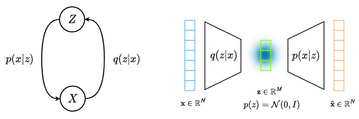
From this graph, we can see that the maximization of the ELBO equation (or the minimization of the above equation) can be handled by an encoder and an decoder!
Let’s work on the decoder
The decoder will be in charge of the optimization of \(p(x \vert z)\), i.e. the first part of the above equation. This is done through a neural network that will optimize the \(f\) function through the minimization of the following loss function:
\[\mathcal{L}_{decoder} = \alpha\|x-\hat{x}\|^2 \,=\, \alpha\|x-\underbrace{f(z)}_{\text{decoder}}\|^2\]where \(f(z)\) is the ouput of the decoder. This correponds to the classical \(L_2\) loss function!
If we make the assumption that \(\,p(x \vert z)\) follows a Bernouilli distribution, then we can demonstrate that the maximization of \(\,\mathbb{E}_{z\sim q_x} \left[log\left(p(x \vert z)\right)\right]\) leads to the minimization of the cross entropy function!
Let’s work on the encoder
The encoder will be in charge of the optimization of \(p(z \vert x)\), i.e. the second part of the above equation. This is done through a neural network that will optimize \(g\) and \(h\) functions through the minimization of the following loss function:
\[\mathcal{L}_{encoder} = D_{KL}(\underbrace{q_x(z)}_{encoder} \parallel \mathcal{N}(0,I))\]A very important point here is that we must think in terms of probability function since we want to fit two distributions. In other words, the encoder must generate the parameters of the distribution that will generate the \(z\) sample.
The execution of the encoder for the same input \(x\) will generate different \(z\) samples whose values should be close to \(\mathcal{N}(0,I)\).
The graph below shows the final network structure used in the VAE formalism.
The following equation is used as a loss term:
\[\text{loss}=\alpha\|x-\hat{x}\|^2 \,+\, D_{KL}\left(\mathcal{N}\left(\mu_x,diag\left(\sigma_x\right)\right),\mathcal{N}\left(0,I\right)\right)\]
And what about backpropagation?
So far, we have established a probabilistic framework that depends on three functions, \(f\), \(g\) and \(h\) that are modeled by neural networks in an encoder-decoder architecture. In practice, g and h are not defined by two completely independent networks but share a part of their architecture and their weights so that we have:
\[g(x)=g_2(g_1(x)) \quad\quad\quad\quad h(x)=h_2(g_1(x))\]Moreover, for simplification purposes, we also make the assumption that \(q_x(z)\) is a multidimensional Gaussian distribution with diagonal covariance matrix (i.e. variables independence assumption). \(h(x)\) is thus simply a vector containing the diagonal elements of the covariance matrix and as the same size as \(g(x)\).

We also need to be very careful about the way we sample from the distribution returned by the encoder during the training.
The sampling process has to be expressed in a way that allows the error to be backpropagated through the network.
A reparametrisation trick is used to make the gradient descent possible despite the random sampling. It consists in using the fact that if \(z\) is a random variable following a Gaussian distribution with mean \(g(x)\) and with covariance \(H(x)=h(x) \cdot h'(x)\) then it can be expressed as:
\[z = h(x) \zeta + g(x) \quad\quad\quad \zeta \sim \mathcal{N}(0,I)\]
This parametrization trick can be summarized as follows:

The graph below shows the final network used to implement VAE with the possibility to perform backpropagation.

We recall that the following equation is used as the loss term:
\[\text{loss} = \alpha\|x-\hat{x}\|^2 \,+\, D_{KL}\left(\mathcal{N}\left(\mu_x,diag\left(\sigma_x\right)\right),\mathcal{N}\left(0,I\right)\right)\] \[\text{loss} = \alpha\|x-f(z)\|^2 \,+\, D_{KL}\left(\mathcal{N}\left(g(x),diag\left(h(x)\right)\right),\mathcal{N}\left(0,I\right)\right)\]