C2FTrans: Coarse-to-Fine Transformers for Medical Image Segmentation
Notes
- Code is available on GitHub: https://github.com/xianlin7/C2FTrans.
Highlights
- Invention of a new transformer architecture, namely Coarse-to-Fine Transformer (C2FTrans), in medical image segmentation. C2FTrans consists of a cross-scale global transformer (CGT) which addresses local contextual similarity in CNN and a boundary-aware local transformer (BLT) which overcomes boundary uncertainty brought by rigid patch partitioning in transformers.
- C2FTrans has only 1.2M parameters.
Architecture
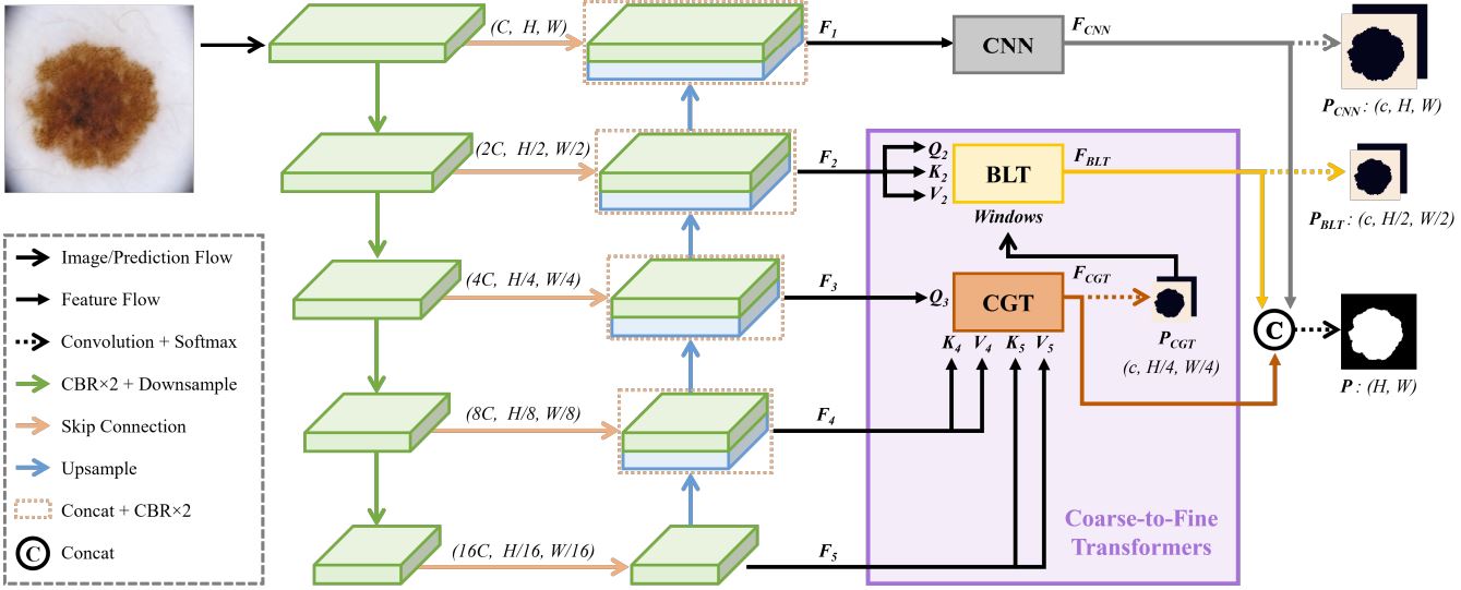 The authors use a full U-Net as backbone for the feature extraction and add transformer modules (CGT and BLT) to the decoder of the U-Net. This idea is quite different from UNETR1 that replaces directly the encoder of the U-Net with transformers.
Cross-scale Global Transformer (CGT)
 CGT is made up of two cross-attention modules and a feed forward network (FFN). CGT aims to mix information coming from the three lowest resolution feature maps, i.e., \(F_3 \in \mathbb{R}^{4 \text{C} \times \frac{\text{H}}{4} \times \frac{\text{W}}{4}}\), \(F_4 \in \mathbb{R}^{8 \text{C} \times \frac{\text{H}}{8} \times \frac{\text{W}}{8}}\), and \(F_5 \in \mathbb{R}^{16 \text{C} \times \frac{\text{H}}{16} \times \frac{\text{W}}{16}}\).
Projections of these three feature maps to obtain \(Q\), \(K\), and \(V\):
- \(F_3\) is projected into query, \(Q_{3,i} \in \mathbb{R}^{\frac{\text{HW}}{16} \times \text{D}_h}\), \(i \in \{4,5\}\), where \(\text{D}_h = 128\) denotes the dimension of the transformer module. A patch size of \((1 \times 1)\) is used for tokenization:
\[F_3 \in \mathbb{R}^{4 \text{C} \times \frac{\text{H}}{4} \times \frac{\text{W}}{4}} \xrightarrow[\text{reshape}]{} \mathbb{R}^{\frac{\text{HW}}{4 \times 4 \times (1 \times 1)} \times ((1 \times 1) \times 4 \text{C})} = \mathbb{R}^{\frac{\text{HW}}{16} \times 4 \text{C}} \xrightarrow[\text{tokenization}]{\mathbb{R}^{4 \text{C} \times \text{D} (=64)}} F^{'}_3 \in \mathbb{R}^{\frac{\text{HW}}{16} \times \text{D}} \xrightarrow[\text{projection}]{\mathbb{R}^{\text{D} \times \text{D}_h}} Q_{3,i} \in \mathbb{R}^{\frac{\text{HW}}{16} \times \text{D}_h}\]
-
\(F_4\) is projected into \(\{K_4, V_4\}\), where \(K_4, Q_4 \in \mathbb{R}^{\frac{\text{HW}}{64} \times \text{D}_h}\).
-
Likewise, \(F_5\) is projected into \(\{K_5, V_5\}\), where \(K_5, Q_5 \in \mathbb{R}^{\frac{\text{HW}}{256} \times \text{D}_h}\).
Cross-scale attention is then obtained by \(F^i_{ca} (Q_{3,i}, K_i, V_i) = \text{softmax}(\frac{Q_{3,i} K^T_i}{\sqrt{\text{d}}}) V_i\), where
\[F^4_{ca} \in (\mathbb{R}^{\frac{\text{HW}}{16} \times \text{D}_h} \times \mathbb{R}^{\text{D}_h \times \frac{\text{HW}}{64}} \times \mathbb{R}^{\frac{\text{HW}}{64} \times \text{D}_h}) = \mathbb{R}^{\frac{\text{HW}}{16} \times \text{D}_h}\] \[F^5_{ca} \in (\mathbb{R}^{\frac{\text{HW}}{16} \times \text{D}_h} \times \mathbb{R}^{\text{D}_h \times \frac{\text{HW}}{256}} \times \mathbb{R}^{\frac{\text{HW}}{256} \times \text{D}_h}) = \mathbb{R}^{\frac{\text{HW}}{16} \times \text{D}_h}\]To be noted that during this step, multiscale features are mixed. According to the authors, this is crucial as lower resolution feature maps correspond to larger receptive fields, hence contain richer semantic information. By extracting \(\text{K}\) and \(\text{V}\) from lower resolution feature maps, computational complexity is reduced by at least a factor of 4 since their sequence length is shorter.
After that, \(F^4_{ca}\) and \(F^5_{ca}\) from all the transformer heads are concatenated and connected residually with \(F^{'}_3\). To do so, another linear projection matrix \(W_{ca} \in \mathbb{R}^{2 \text{gD}_h \times \text{D}}\) is learned, where \(\text{g}\) represents the number of self-attention heads:
\[\begin{align} F_{ca} &= \underbrace{\text{concat}(F^4_{ca,1}, \cdots, F^4_{ca,g}, F^5_{ca,1}, \cdots, F^5_{ca,g})}_{\mathbb{R}^{\frac{\text{HW}}{16} \times \text{D}_h \times \text{2g}} \xrightarrow[\text{reshape}]{} \mathbb{R}^{\frac{\text{HW}}{16} \times \text{2gD}_h}} \cdot \overbrace{W_{ca}}^{\mathbb{R}^{2 \text{gD}_h \times \text{D}}} + F^{'}_3 \in \mathbb{R}^{\frac{\text{HW}}{16} \times \text{D}} \\ F_{ca} &= \text{FFN}(F_{ca}) + F^{'}_3 \\ \end{align}\]To obtain the final CGT output, \(F_{CGT}\):
\[F_{ca} \in \mathbb{R}^{\frac{\text{HW}}{16} \times \text{D}} \xrightarrow[\text{reshape}]{} \mathbb{R}^{\text{D} \times \frac{\text{H}}{4} \times \frac{\text{W}}{4}} \xrightarrow[1 \times 1 \text{ conv}]{} F_{CGT} \in \mathbb{R}^{\text{D} \times \frac{\text{H}}{4} \times \frac{\text{W}}{4}}\]
⚠️ In the paper, it is written that they learn two projection matrices and apply a residual connection to get \(F_{CGT}\), which contradicts their GitHub code.
\(F_{CGT}\) is then transformed for the downstream tasks:
- Computation of boundary-aware windows for BLT.
- Generation of a low-resolution mask for multiscale loss computation.
- Generation of a probability map of initial image dimension (via upsampling) that will be concatenated with the another two probability maps from U-Net and BLT to form the final probability map.
Boundary-aware Local Transformer (BLT)
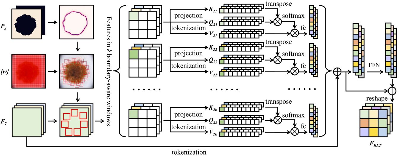
According to the authors, the rigid patch partitioning of transformer destroys the vital details around boundaries. Hence, the core contribution of BLT is to perform local self-attention within boundary-aware windows.
Generation of boundary-aware windows:
1) Create evenly and densely tiled windows over feature map \(F_2 \in \mathbb{R}^{2\text{C} \times \frac{\text{H}}{2} \times \frac{\text{W}}{2}}\) to obtain an initial window set \(\{w \}\).
2) Calculate entropy of each pixels in \(P_{CGT}\). These entropies are then used to compute the scores for each window. This can help to effectively localize the boundary windows as positions with higher entropy scores are more likely to be real boundaries.
3) Apply non-maximum suppression to keep the highest score windows and discard overlapping boxes. A filtered window set \(\{w^{*} \}\) is obtained.
4) Align \(\{w^{*} \}\) with \(F_2\) to form the corresponding feature map \(\{f^{*} \}\).
Projections of \(\{f^{*} \}\) to obtain \(Q_{2,k}\), \(K_{2,k}\), and \(V_{2,k}\), where \(k\) denotes the number of windows. The size of each window is fixed at \(16 \times 16\):
\[f^{*} \in \mathbb{R}^{(16 \times 16) \times 2\text{C}} \xrightarrow[\text{tokenization}]{\mathbb{R}^{2 \text{C} \times \text{D}}} \mathbb{R}^{(16 \times 16) \times \text{D}} \xrightarrow[\text{projection}]{\text{E}_{q,k,v} \in \mathbb{R}^{\text{D} \times \text{D}_h}} Q_{2,k}, K_{2,k}, V_{2,k} \in \mathbb{R}^{(16 \times 16) \times \text{D}_h}\]For each window, the self-attention is computed. The authors do not mention how these self-attention maps are combined. The combined attention maps with the residual connection with the tokenized \(F_2\) will then be fed to a FFN to obtain \(F_{sa,i}, i \in \{1 \cdots \text{g}\}\), where \(\text{g}\) is the number of transformer heads. Afterwards, the outputs of all the heads are concatenated to form \(F_{sa}\). Just like the CGT, the final BLT output, \(F_{BLT}\) will be used to generate the low-res probability map for loss computation and upsampled to produce the full scale probability map.
Some training parameters
- Multiscale loss with specific weights:
- Smooth L1 loss
- Dice loss
- Cross-entropy loss
- 400 training epochs
- Adam optimizer
- ReduceLROnPlateau
- Input images resized to \(256 \times 256\)
Benchmarking datasets
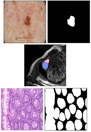
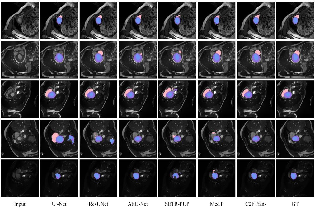
The authors test their network on three datasets: ISIC 2018 (2596 images for lesion segmentation), ACDC (150 cardiac MR 3D images), and GLaS (165 microscopic images of hematoxylin and eosin-stained slides).
Results
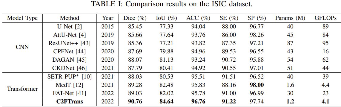
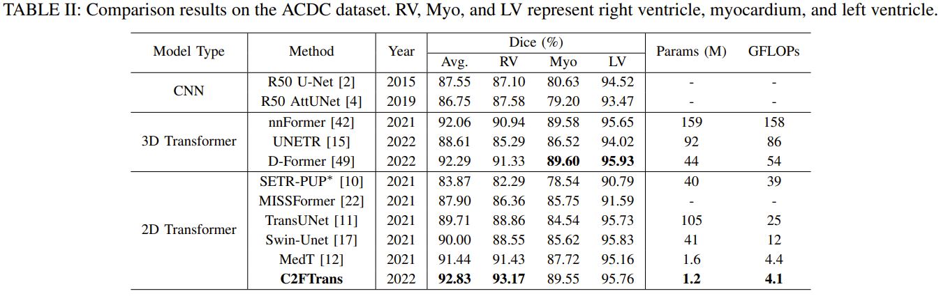
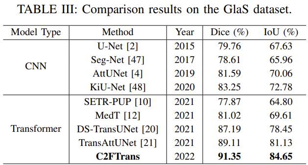
The authors mention the comparison between the SOTA methods but it lacks the comparison with nnUNet and swin-UNETR, the two most powerful segmentation algorithms.
Conclusions
The introduction of C2F transformer in medical image segmentation is interesting, especially the Cross-scale Global Transformer. However, their GitHub repository is not easy to use. I had a hard time setting up the correct environment. I have also tested their algorithm on the Camus dataset and the results were worse than those given by nnUNet.
References
-
Review of “UNETR: Transformers for 3D Medical Image Segmentation”: https://creatis-myriad.github.io/2022/07/01/UNETR-TransformerMedicalImageSegmentation.html ↩