A probabilistic U-Net for the segmentation of ambiguous images
Notes
Highlights
- The objective of this paper is to learn a distribution of segmentations from an input.
- The main innovation concerns the design of a generative segmentation model based on the combination of a U-Net with a conditional VAE.
- The proposed framework is also capable of learning hypotheses that have a low probability and predicting them with the corresponding frequency.
Method
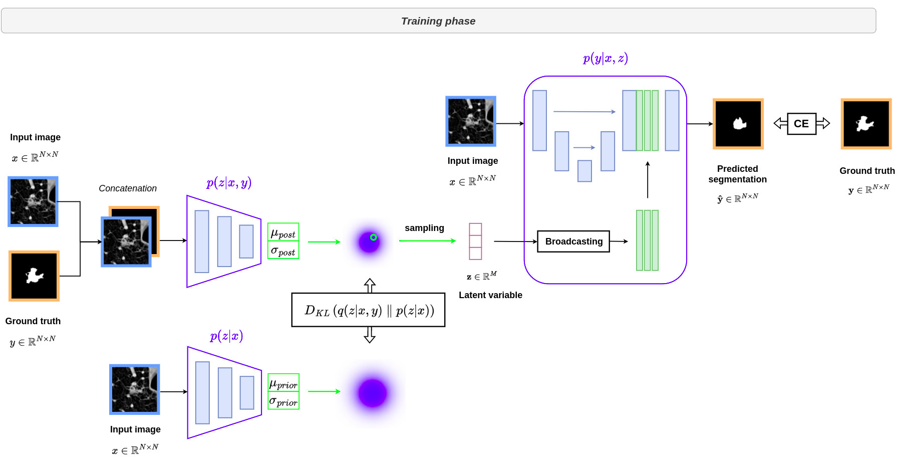
Architecture
- The architecture is based on the conditional VAE whose details are provided in the following tutorial.
- The innovation comes from the use of a U-Net architecture to model the distribution \(p(y \vert x,z)\).
- The latent vector \(z\) is first broadcast to produce a \(N\)-channel feature map with the same spatial dimensions as the segmentation map. This feature map is then concatenated with the last activation map of a U-Net before being convolved by a last layer to produce the final segmentation map with the desired number of classes.
The image below provides an overview of the architecture deployed during training. The distributions \(p(z \vert x,y)\), \(p(z \vert x)\) and \(p(y \vert x,z)\) displayed in blue are modeled by three distinct neural networks.
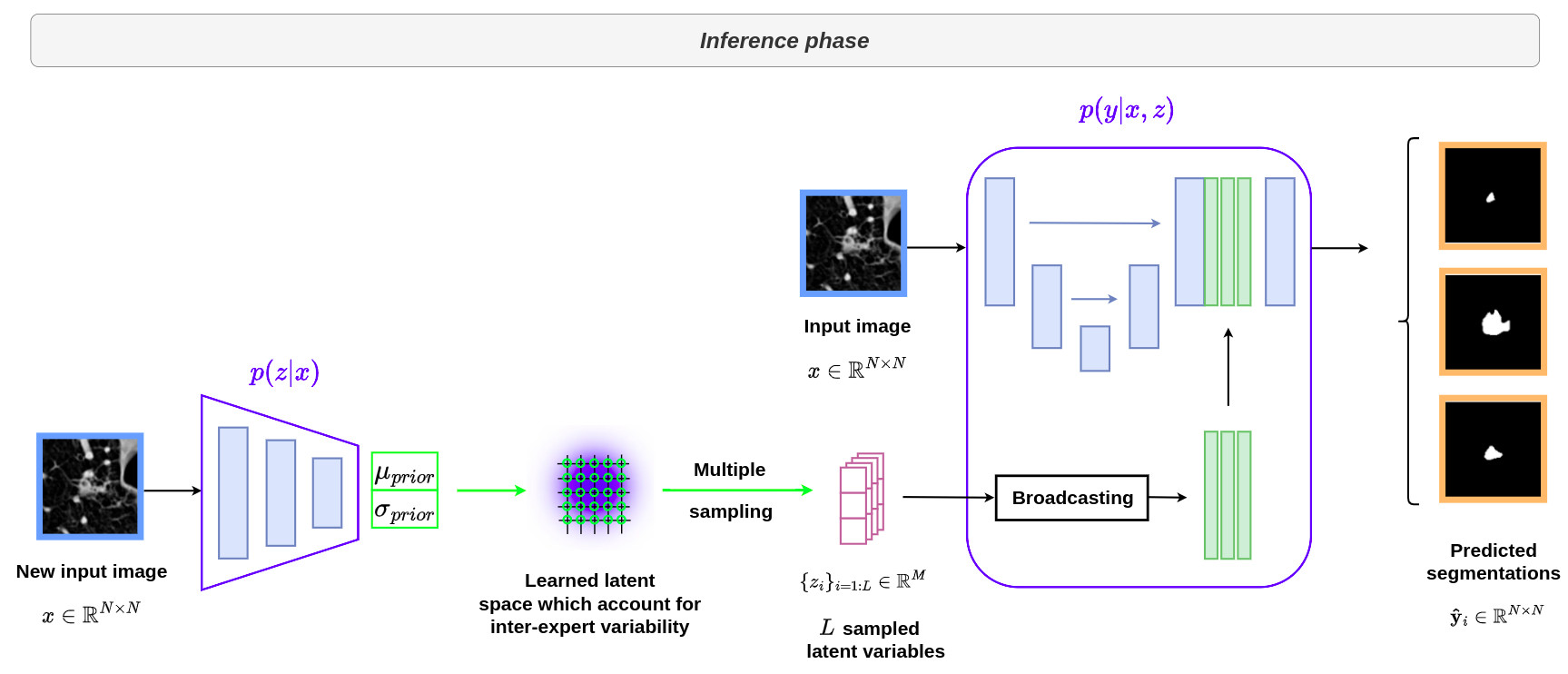
The following image illustrates the use of the architecture during inference.
Implementation details
- The dimensions of the latent space has been experimentally fixed at \(M=6\) and is kept fixed in all experiments.
- The difference between the predicted segmentation and the ground truth is optimized using a Cross Entropy loss.
- The training is done from scratch with randomly initialized weights
- When drawing \(m\) samples for the same input image, the output of the prior network and the feature activations of the U-Net can be reused without the need for recomputation, making the overall strategy computationally efficient.
Performance measures
- The performance of the methods was evaluated by comparing distributions of segmentations.
- This was done through the computation of generalized energy distance whose expression is given below:
- \(d\) is a distance measure, \(y\) and \(y'\) are independent samples from the ground truth distribution \(P_{gt}\), \(\hat{y}\) and \(\hat{y}'\) are independent samples from the predicted distribution \(P_{out}\).
- The distance measure is based on the \(IoU\) metric and is defined as follows: \(d(x,y)=1-IoU(x,y)\).
Results
LIDC-IDRI dataset
- 1010 2D+slices CT scan of lungs with lesions
- For each scan, 4 radiologists (from a total of 12) provided annotation masks for lesions that they independently detected
- the CT scans were resampled to \(0.5 \, \text{mm} \times 0.5 \, \text{mm}\) in-plane resolution and cropped 2D images (\(180 \times 180\) pixels) centered at the lesion positions.
- This resulted in \(8882\) images in the training set, \(1996\) images in the validations set and \(1992\) images in the test set.
- Because the experts can disagree, up to 3 masks per image can be empty.
As shown in the figure below, the probabilistic U-Net network outperforms state-of-the-art methods in effectively representing the ground truth distribution.

Analysis of the latent space
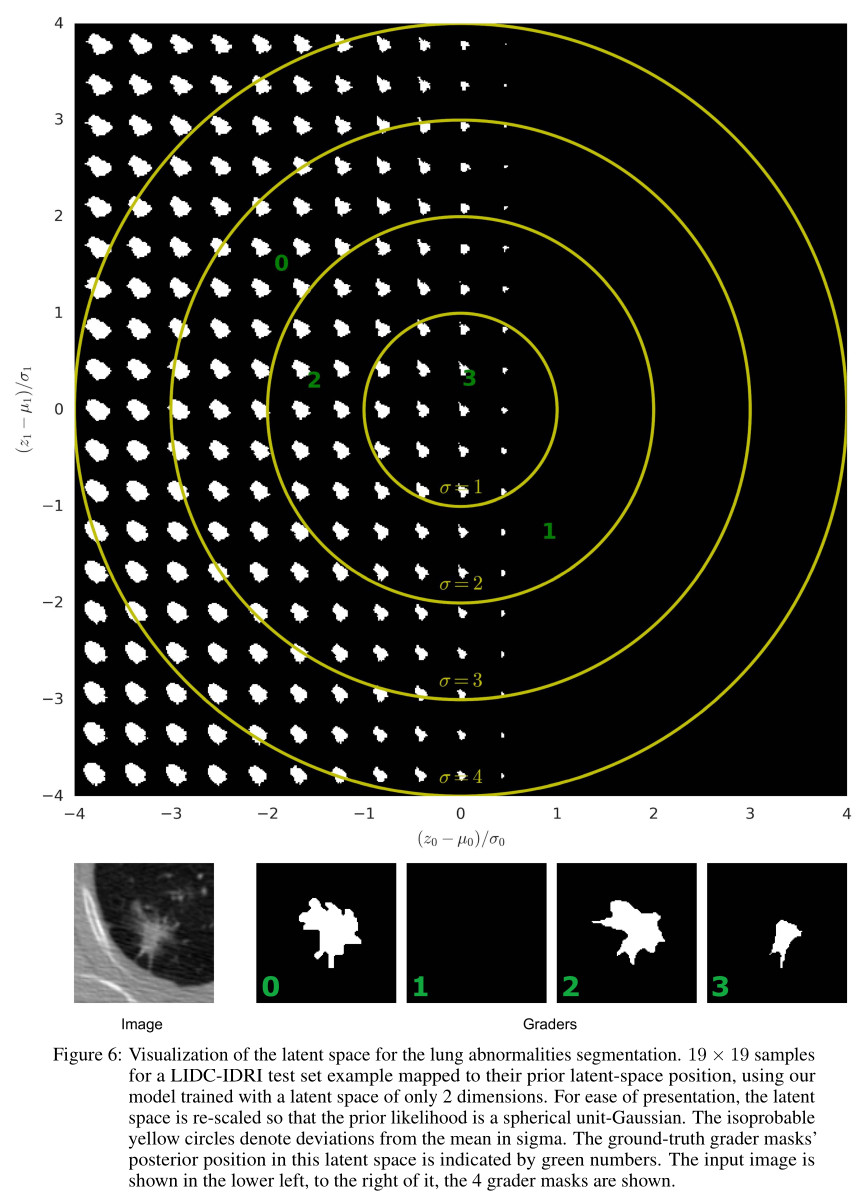
- The authors proposed to visualize the latent space by arranging the samples to represent their corresponding position in a 2D plane, i.e. the dimension of the latent space was set to \(2\) and each latent variable was normalized by the inferred mean and standard deviation computed from the tested image: \(\hat{z}=\left(z-\mu\right)/\sigma\).
- This allows to interpret how the model ends up structuring the space to solve the given tasks.
- The latent space given in the figure below was computed from a specific image, where 3 over 4 annotators provided a segmentation
- The part of the latent space included in the \(\sigma=1\) circle indicates the most probable generated masks. This region clearly shows that the algorithm has taken into account the occurrence of the images segmented by the experts: there is more chance to generate a segmentation mask than an empty image.
- From this figure, one can see that the \(z_0\) component encodes lesion size including a transition to complete lesion absence, while the \(z_1\) component encodes shape variations.
Some examples and needs for improvement
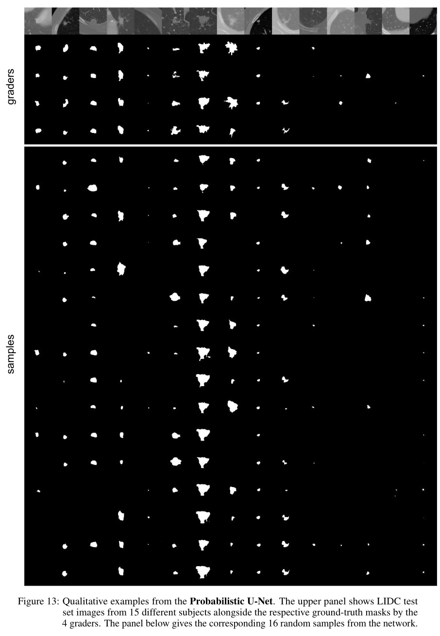
The figure below shows some examples of segmentations generated from the proposed method. From this figure, it can be seen that:
- (good point) the global shapes drawn by the experts are well respected in the generated segmentations.
- (bad point) cases with absence of lesion can be generated even if all the experts have proposed a segmentation mask for the same lesion.
Conclusions
- The authors of this paper have proposed a mixing of U-Net and conditional VAE to design a generative network that learns the variability of hand-drawn shapes by several experts.
- Even if the fomalism provides interesting results, there is room for improvement in results.
- The same authors have proposed an improved version of this formalism called hierarchical probabilistic U-Net. This method will be studied in a future post!