What about the conditional variational autoencoder?
Notes
-
This tutorial was mainly inspired by the following two papers: Sohn et al., NeurIPS 2015 and Kohl et al., NeurIPS 2018.
- Introduction
- Variational inference
- Various scenarios
- Simple example
Introduction
Conditional variational autoencoders (cVAE) should not been seen as an extension of conventional VAE! cVAE are also based on variational inference, but the overall objective is different:
- In the VAE formalism, a pipeline is optimized to produce outputs as close as possible to the input data in order to build an efficient latent space with reduced dimensionality. This latent space is then used during inference for interpretation purposes.
- In the cVAE formalism, a pipeline is optimized to build a latent space that captures reference variability. This latent space is then used in inference to generate a set of plausible outputs for a given input \(x\).
VAE
A complete tutorial on VAEs can be found here. The graph below summarizes the overall strategy used in VAE formalism during training.

The goal of VAEs is to learn an embedding (latent) space that efficiently represents the distribution of the \(x\) input in a lower dimensional space for easier interpretation.
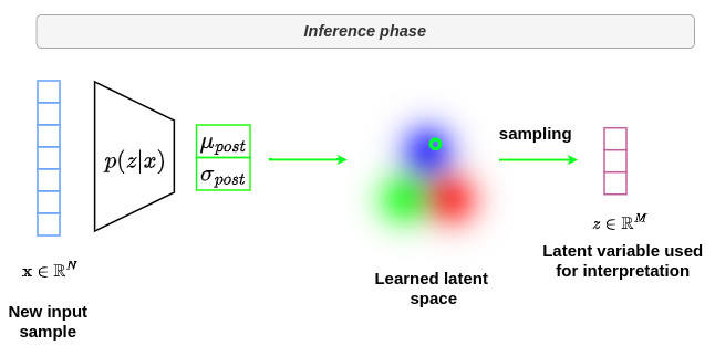
During inference, a new input \(x\) is given as input to the encoder \(p(z \vert x)\) and a dedicated analysis can be performed within the latent space.
cVAE
In comparison, the two graphs below shows the overall strategy used in the conditional VAE formalism during training and inference, respectively.
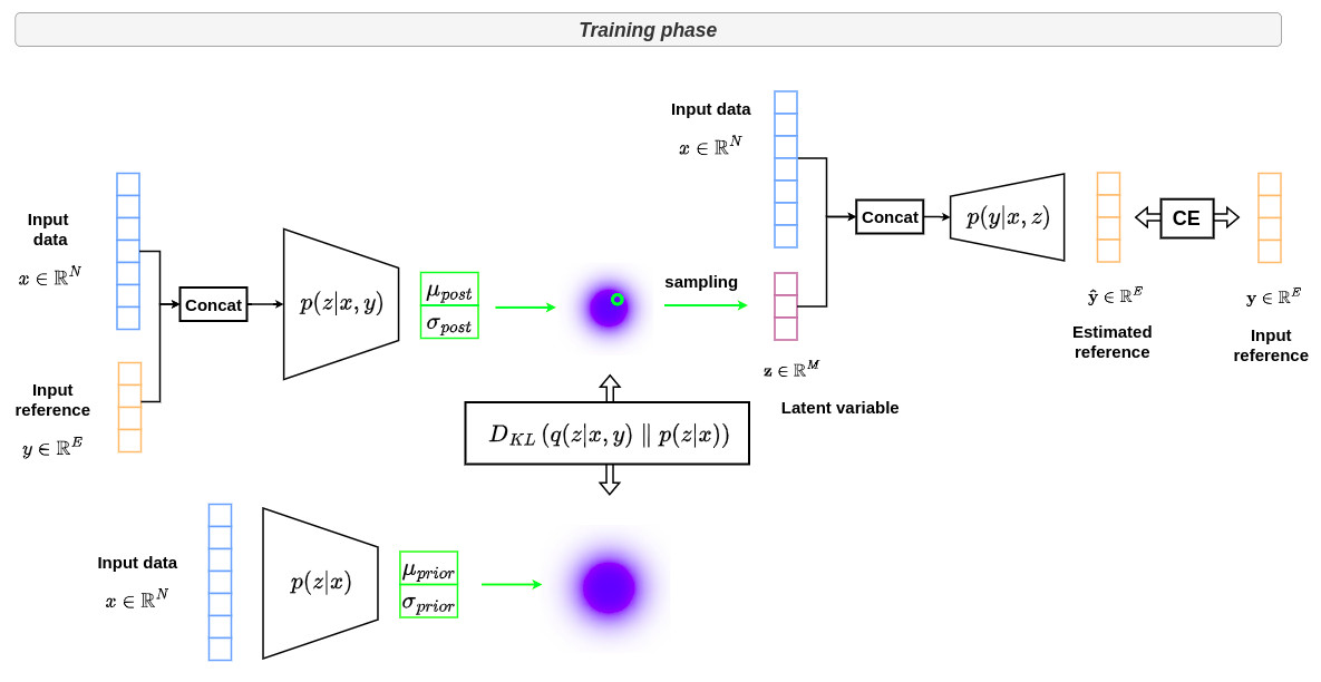
The goal of conditional VAE is to learn an embedding (latent) space that efficently captures the reference variability in a space with reduced dimensionality.
This is achieved by learning the distribution \(p(z \vert x,y)\) which generates a latent space that embeds joint effective information from \(x\) and \(y\).
In parallel, the prior network learns to match this distribution by learning \(p(z \vert x)\) through the Kullback-Liebler (KL) divergence. The interest of this network after training is that we no longer need \(y\) to get the mapping from \(x\) to the corresponding latent space. This will be very useful for inference.

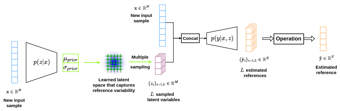
During inference, a new sample \(x\) is given as input to \(p(z \vert x)\) and several points \(z_i\) are sampled in the corresponding latent space to generate a set of plausible outputs \(\hat{y}_i\) that will represent the learned variability of the references for a given \(x\).
Variational inference
Overall strategy
The goal of conditional VAE is to approximate a \(p(y \vert x)\) distribution through a latent space that captures the variability of references by learning the \(p(z \vert x,y)\) distribution. This way, the distribution \(p(y \vert x,z)\) will allow to generate multiple plausible references from a given \(x\). The following scheme is applied:
- for a given observation \(x\), a set of latent variables \(z_i\) is generated from \(p(z \vert x,y)\) thanks to the sampling of the latent space posterior.
- The set of latent variables are then combined with the observation \(x\) and passed through the conditional generative process \(p(y \vert x,z)\) to generate samples from the distribution \(y\).
- The resulting predictive distribution is finally obtained through the following expression:
As for the variational autoencoders, the key challenge around conditional VAE is the computation of the posterior \(p(z \vert x,y)\). Indeed, due to intractable properties, the derivation of this distribution is complicated and requires the use of approximation techniques such as variational inference.
In the conditional VAE formalism, the posterior \(p(z \vert x,y)\) is modeled as an axis-aligned Gaussian distribution \(q(z \vert x,y)\) whose mean \(\mu_{post}\) and covariance \(\sigma_{post}\) are defined by two functions \(g(x,y)\) and \(h(x,y)\).
\[q(z \vert x,y) = \mathcal{N}\left(\mu_{post},diag\left(\sigma_{post}\right)\right) = \mathcal{N}\left(g(x,y),diag\left(h(x,y)\right)\right)\]We thus have a family of candidates for variational inference and need to find the best approximation among this family by minimizing the KL divergence between the approximation \(q(z \vert x,y)\) and the target \(p(z \vert x,y)\). In other words, we are looking for the optimal \(g^∗\) and \(h^∗\) functions such that:
\[\left(g^*,h^*\right) = \underset{(g,h)}{\arg\min} \,\,\, D_{KL}\left(q(z \vert x,y) \parallel p(z \vert x,y) \right)\]
One particularity of the conditional VAE formalism is that the distribution \(p(z \vert x)\) is also modeled as an axis-aligned Gaussian distribution \(p(z \vert x)\) whose mean \(\mu_{prior}\) and covariance \(\sigma_{prior}\) are defined by two functions \(k(x,y)\) and \(l(x,y)\).
\(p(z \vert x)\) is thus modeled as:
\[p(z \vert x) = \mathcal{N}\left(\mu_{prior},diag\left(\sigma_{prior}\right)\right) = \mathcal{N}\left(k(x,y),diag\left(l(x,y)\right)\right)\]As we will see later, minimizing the KL divergence between the approximation \(q(z \vert x,y)\) and the target \(p(z \vert x,y)\) also leads to finding the optimal \(k^*\) and \(l^*\) functions.
Formulation of the KL divergence
Let’s now reformulate the KL divergence expression
\[D_{KL}\left(q(z \vert x,y) \parallel p(z \vert x,y) \right) = - \int{q(z \vert x,y) \cdot log\left(\frac{p(z \vert x,y)}{q(z \vert x,y)}\right) \,dz}\]Using the following conditional probability relations:
\[p(x,y,z) = \left\{ \begin{array} pp(y,z \vert x) \cdot p(x) \\ p(z \vert x,y) \cdot p(x,y) \end{array} \right.\] \[p(x,y) = p(y \vert x) \cdot p(x)\]the next equations can be easily obtained
\[p(z \vert x,y) = \frac{p(y,z \vert x) \cdot p(x)}{p(x,y)}\] \[p(z \vert x,y) = \frac{p(y,z \vert x) \cdot p(x)}{p(y \vert x) \cdot p(x)}\] \[p(z \vert x,y) = \frac{p(y,z \vert x)}{p(y \vert x)}\]
The previous KL divergence expression can thus be rewritten as
\[D_{KL}\left(q(z \vert x,y) \parallel p(z \vert x,y) \right) = - \int{q(z \vert x,y) \cdot log\left(\frac{p(y,z \vert x)}{p(y \vert x) \cdot q(z \vert x,y)}\right) \,dz}\] \[= - \int{q(z \vert x,y) \cdot \left[log\left(\frac{p(y,z \vert x)}{q(z \vert x,y)}\right) + log\left(\frac{1}{p(y \vert x)}\right) \right]\,dz}\] \[= - \int{q(z \vert x,y) \cdot log\left(\frac{p(y,z \vert x)}{q(z \vert x,y)}\right)\,dz} + log\left(p(y \vert x)\right) \cdot \underbrace{\int{q(z \vert x,y)\,dz}}_{=1}\] \[D_{KL}\left(q(z \vert x,y) \parallel p(z \vert x,y) \right) \,+\, \mathcal{L} \,=\, log\left(p(y \vert x)\right)\]where \(\mathcal{L}\) is defined as the Evidence Lower BOund (ELBO), whose expression is given by:
\[\mathcal{L} = \int{q(z \vert x,y) \cdot log\left(\frac{p(y,z \vert x)}{q(z \vert x,y)}\right) \,dz}\]
Evidence lower bound
Let’s take a closer look at the previous derived equation:
\[D_{KL}\left(q(z \vert x,y) \parallel p(z \vert x,y) \right) \,+\, \mathcal{L} \,=\, log\left(p(y \vert x)\right)\]The following observations can be made:
-
since \(0\leq p(y \vert x) \leq 1\), then \(log\left(p(y \vert x)\right) \leq 0\)
-
since \(x\) and \(y\) are known, then \(log\left(p(y \vert x)\right)\) is a fixed value
-
by definition \(D_{KL}\left(q(z \vert x,y) \parallel p(z \vert x,y) \right) \geq 0\)
-
since \(\mathcal{L} = -D_{KL}\left(q(z \vert x,y) \parallel p(y,z \vert x)\right)\), then \(\mathcal{L} \leq 0\)
The previous expression can thus be rewritten as follows:
\[\underbrace{D_{KL}\left(q(z \vert x,y) \parallel p(z \vert x,y) \right)}_{\geq 0} \,+\, \underbrace{\mathcal{L}}_{\leq 0} \,=\, \underbrace{log\left(p(y \vert x)\right)}_{\leq 0 \,\, \text{and fixed}}\]Thus, by tweaking \(q(z \vert x,y)\), we can seek to maximize the ELBO \(\mathcal{L}\), which will imply the minimization of the KL divergence \(D_{KL}\left(q(z \vert x,y) \parallel p(z \vert x,y) \right)\), and consequently a distribution \(q(z \vert x,y)\) that is close to \(p(z \vert x,y)\).
ELBO reformulation
The ELBO \(\mathcal{L}\) must be reformulated to derive the loss involved in the conditional VAE framework. The corresponding derivation is provided below:
\[\mathcal{L} = \int{q(z \vert x,y) \cdot log\left(\frac{p(y,z \vert x)}{q(z \vert x,y)}\right) \,dz}\]By using the following conditional probability relations:
\[p(x,y,z) = \left\{ \begin{array} pp(y,z \vert x) \cdot p(x) \\ p(y \vert x,z) \cdot p(x,z) \end{array} \right.\] \[p(x,y) = p(z \vert x) \cdot p(x)\]the next equations can be easily obtained
\[p(y,z \vert x) = \frac{p(y \vert x,z) \cdot p(x,z)}{p(x)}\] \[p(y,z \vert x) = \frac{p(y \vert x,z) \cdot p(z \vert x) \cdot p(x)}{p(x)}\] \[p(y,z \vert x) = p(y \vert x,z) \cdot p(z \vert x)\]
The ELBO \(\mathcal{L}\) expression can thus be rewritten as
\[\mathcal{L} = \int{q(z \vert x,y) \cdot log\left(\frac{p(y \vert x,z) \cdot p(z \vert x)}{q(z \vert x,y)}\right) \,dz}\] \[\mathcal{L} = \int{q(z \vert x,y) \cdot \left[log\left(p(y \vert x,z)\right) + log\left(\frac{p(z \vert x)}{q(z \vert x,y)}\right) \right] \,dz}\] \[\mathcal{L} = \int{q(z \vert x,y) \cdot log\left(p(y \vert x,z)\right) \,dz} \,+\, \int{q(z \vert x,y) \cdot log\left(\frac{p(z \vert x)}{q(z \vert x,y)}\right) \,dz}\] \[\mathcal{L} = \mathbb{E}_{z\sim q(z \vert x,y)} \left[log\left(p(y \vert x,z)\right)\right] - D_{KL}\left(q(z \vert x,y)\parallel p(z \vert x)\right)\]where \(\mathbb{E}_{z\sim q(z \vert x,y)}\) is the mathematical expectation with respect to \(q(z \vert x,y)\).
At this stage of analysis, it is important to note that \(p(y \vert x,z)\) will be approximated by a neural network \(f(\cdot)\) so that \(\hat{y}=f(x,z)\). Since this function is deterministic, it will allow to model \(p\left(y \vert \hat{y}\right)\). By approximating \(p\left(y \vert \hat{y}\right)\) by a Bernoulli distribution, we have
\[\mathbb{E}_{z\sim q(z \vert x,y)} \left[log\left(p(y \vert \hat{y})\right)\right] = \mathbb{E}_{z\sim q(z \vert x,y)} \left[log\left( {\hat{y}}^y \cdot \left(1-\hat{y}\right)^{1-y} \right)\right]\] \[= \mathbb{E}_{z\sim q(z \vert x,y)} \left[ y \, log\left( \hat{y} \right) + \left(1-y\right) \, log\left(1-\hat{y}\right) \right]\] \[= \mathbb{E}_{z\sim q(z \vert x,y)} \left[-CE\left( y,f\left(x,z\right)\right)\right]\]where \(CE(\cdot)\) corresponds to the conventional cross entropy function !
Following this modeling, we are finally looking for:
\[\left(f^*,g^*,h^*,k^*,l^*\right) = \underset{(f,g,h,k,l)}{\arg\max} \,\,\, \left( \mathbb{E}_{z\sim q(z \vert x,y)} [-CE\left( y,f\left(x,z\right)\right)] - D_{KL}(\underbrace{q(z \vert x,y)}_{g,h}\parallel \underbrace{p(z \vert x)}_{k,l}) \right)\]which is equivalent to
\[\left(f^*,g^*,h^*,k^*,l^*\right) = \underset{(f,g,h,k,l)}{\arg\min} \,\,\, \left( \mathbb{E}_{z\sim q(z \vert x,y)} [CE\left( y,f\left(x,z\right)\right)] + D_{KL}(\underbrace{q(z \vert x,y)}_{g,h}\parallel \underbrace{p(z \vert x)}_{k,l}) \right)\]
Various scenarios
There are different ways to leverage the cVAE formalism depending on the modeling of \(p(z \vert x)\) and the content of the \(y\) references.
Modeling of \(p(z \vert x)\)
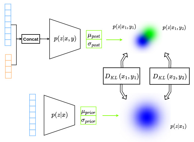
- The distribution \(p(z \vert x)\) outputs a latent variable \(z\) depending on the input \(x\). This means that the corresponding latent space will be structured according to a varying input \(x\) as illustrated in the figure below.
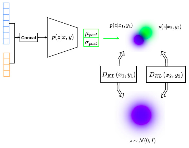
- Several works in the literature propose to relax this constraint to make the latent variables statistically independent of input variables, i.e. \(p(z \vert x) = p(z)\) with \(z \sim \mathcal{N}\left(0,I\right)\). This implies that the latent space is forced to be centered at the origin with unit variance, which makes the posterior modeling strategy close to that used in standard VAE, as illustrated in the figure below.
Nature of the references
Depending on the type of reference available, the value of conditional VAE can be different.
- If there exists only one reference for a given input, the interest of the conditional VAE resides in the mixing of the input \(x\) data with the corresponding \(y\) in the latent space through the modeling of \(p(z \vert x,y)\). This can be viewed as a regularisation process that “efficiently” integrates reference information during inference thanks to the dedicated latent space and the mapping \(p(y \vert x,z)\).
In the context of segmentation, modeling \(p(z \vert x,y)\) can be seen as an “efficient” way to integrate shape prior into the latent space.
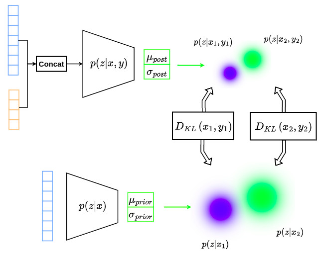
- If there exists several references for a given input, which is the case when we want to model inter/intra-expert variability, the interest of the conditional VAE resides in its capacity to model the reference variability in the latent space through the modeling of \(p(z \vert x,y)\) and the integration of completeness through the modeling of \(p(z \vert x)\). This way, a single input corresponds to several latent variables that are located in the same region of the space, as illustrated in the figure below.
During inference, the latent space modeled by the prior network is sampled several times to generate multiple plausible references \(\hat{y}_i\) from a given input \(x\), taking into account the learned variability as shown in the figure below.
In the context of segmentation, this approach is useful for learning inter-expert variability.
Simple example
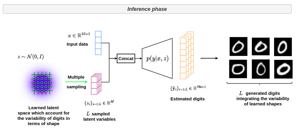
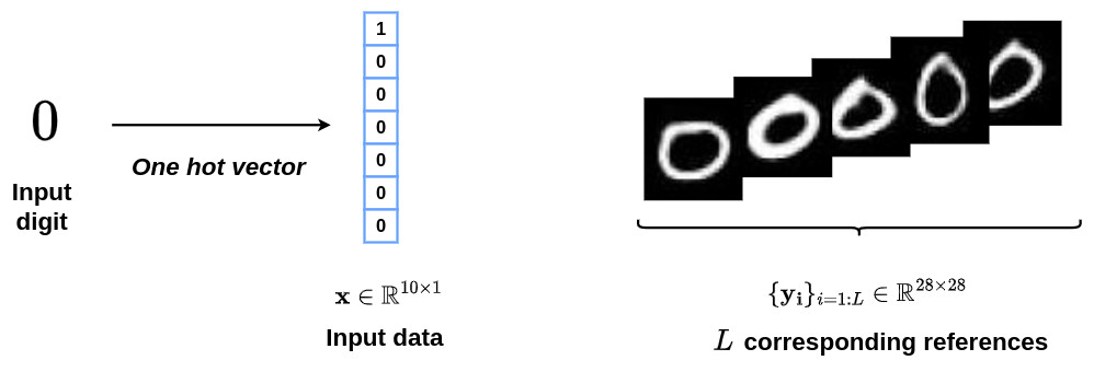
In this example, we will use the conditional VAE formalism to model the variability of handwritten digits. In this context, the input \(x\) refers to a one-hot vector of a specific digit and \(\{y_i\}_{i=1:L}\) refers to the corresponding handwritten images, as shown in the figure below.
Thanks to the conditional VAE formalism, the variability of the manual tracing of the digits is captured during the learning phase through the following architecture.
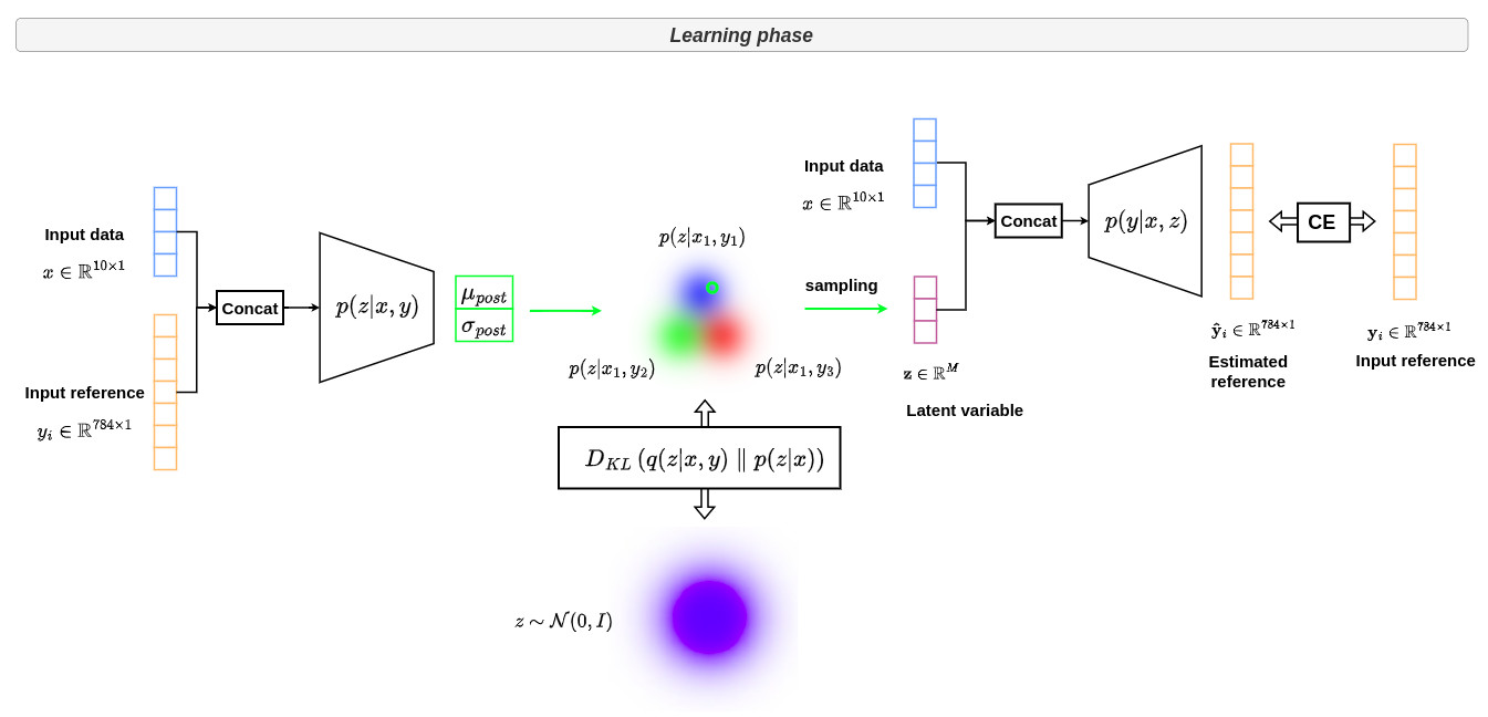
During inference, a digit is given as input to \(p(z \vert x)\) and several \(z_i\) are sampled in the corresponding latent space. This generates a set of plausible output digits \(\hat{y}_i\) integrating the variability of learned shapes, as illustrated below.