DALL-E 2 explained
Highlights
- unCLIP, most commonly known as DALL-E 2, is a generative model that leverage the powerful CLIP joint image and text embedding.
- It is composed of two main components : a prior that convert a CLIP text embedding into a CLIP image embedding and a decoder whose goal is the reverse the CLIP image encoder to produce an output image.
- DALL-E 2 can be tested on this page
unCLIP overview
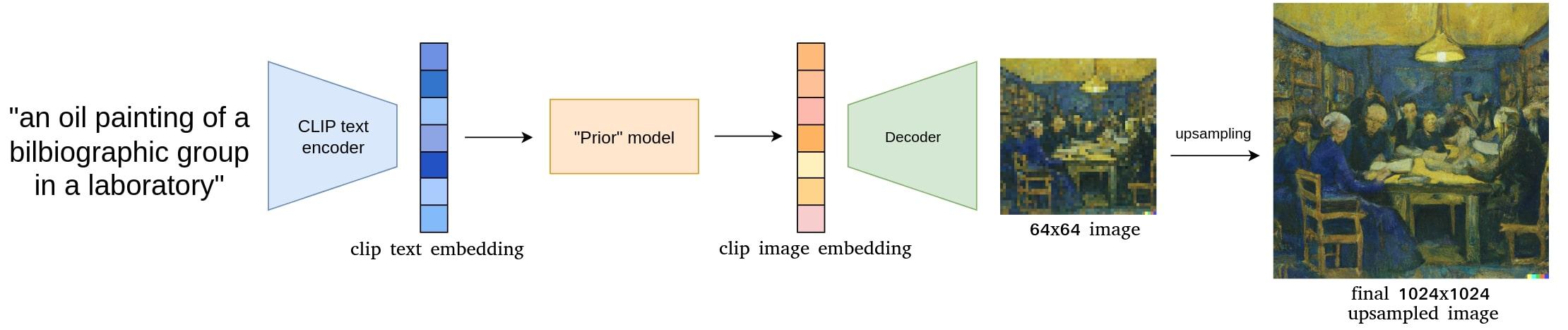
Figure 1.Overview of unCLIP model.
unCLIP uses the power of CLIP as a joint image and text encoder trained on more thant 400 millions of pairs \((x,y)\) of data, respectively an image and its associated caption. Let denote \(z_i\) and \(z_t\) the image and text embeddings. CLIP is trained to produce an image from a caption thanks to two main components :
- a prior \(P(z_i \vert y)\) that predicts an image embedding from a caption (or similarilly from its unique associated text embedding \(z_t\))
- a decoder \(P(x \vert z_i, y)\) that reverse the CLIP image encoding process to produce an image from the predicted image embedding.
The output of the decoder is of size 64x64 and it takes two upsampling models to get to the final resolution (64x64 -> 256x256 and 256x256 -> 1024x1024).
An important part is that the image generation is not (only) conditionned by the caption but it uses the authors found that using CLIP embeddings gave better results. Examples of results are shown later in the review.
- CLIP model uses a ViT-H/16 image encoder with 256x256 images, a width of 1280 and 32 Transformer blocks.
- The CLIP text encoder is a Transformer with causal attention mask, width of 1024 and 24 transformer blocks.
- Encoder is trained with data from CLIP and DALL-E dataset (~ 650M images)
- Prior, decoder and upsamplers are only trained with the DALL-E dataset (~250M images)
Even if unCLIP is called ‘DALL-E 2’, the way it works is very different from the first version of DALL-E (based on VQ-VAE).
Prior
The authors have trying two different models for the prior, an autoregressive model, and a diffusion models. Both showed similar results but the latter was more computationnally efficient so it is the one that was kept (the details of how the AR was used will thus not be detailed here).
A diffusion model aims to generate data from a target distribution from pure Gaussian noise. The process can be seen as a Markov chain during which at each step, the data is corrupted by a small amount of noise. A diffusion model is trained to reverse this corrupting process (see this tutorial for more detailled explanations).
- The diffusion model used here is a decoder’s Transformer1 with causal attention mask, width of 1664 and 24 blocks.
- The sequence of tokens used is the following : the encoded text \(y\), the CLIP text embedding \(z_t\), an embedding for the diffusion timestep, the noised CLIP image embedding whose output at the end of the diffusion process will then be used in the decoder.
- Training objective function : \(L_{prior} = \mathbb{E}_{t \sim [1,T], z_i^{(t)} \sim q_t} [ \lVert f_{\theta} (z_i^{(t)}, t, y) - z_i \rVert_2^2 ]\).
- To improve sampling quality, two samples of \(z_i\) are predicted and only the one with the higher dot product with \(z_t\) is kept.
Note that the model aims to predict directly the unnoised \(z_i\) and not the noise like it is most commonly done in diffusion models.
Decoder
The decoder is greatly inspired from GLIDE2, a previous text-guided generative diffusion model developed by OpenIA.
- The diffusion is a DDIM (Denoising Diffusion Implicit Model3), not a standard DDPM. It has two main features : allowing faster sampling without loss of quality and it has an additional parameter \(\eta\) such that the generation is deterministic when \(\eta=0\) and stochastic when \(\eta > 0\) (and it is equivalent to DDPM when \(\eta=1\))
- The architecture used for the diffusion is a UNet with Attention layers.
- First conditioning : time encoding + last token of the text embedding + projection of the CLIP image embeddings. Passed into the residual blocks of the UNet.
- Second conditioning : Tokens from CLIP text encoder concatenated with 4 tokens coming from the projection of CLIP image embeddings. Concatenated to the keys and values of attention layers of the UNet.
- The conditioned UNet diffusion model has 3.5 billions parameters.
- Classifier-free guidance4 by randomly setting the CLIP embeddings and the text caption embeddings to zeros with a respective probability of 10% and 50%.
Note : classifier-free guidance gives two possible outputs at each diffusion step : \(\epsilon_\theta (x_t \vert c)\) (conditioned output) \(\epsilon_\theta (x_t \vert \emptyset)\) (unconditioned output). During sampling, the output of the model is get via : \(\hat{x}_\theta(x_t \vert y) = \epsilon_\theta(x_t \vert \emptyset) + s \cdot (\epsilon_\theta(x_t \vert t) - \epsilon_\theta(x_t \vert \emptyset))\) with \(s > 1\) (found empirically).

Figure 2. Detailed architecture of the prior and the decoder.
Importance of the prior
The prior and the conditioning on the estimated CLIP image embeddings is one of the main add from the previous OpenIA image generation model. They found that the obtained results are comparable in quality compared to GLIDE but with greater diversity and context understanding.

Figure 3. Examples of images generated by DALL-E 2.
Upsamplers
- Two upsamplers : 64x64 -> 256x256 and 256x256 -> 1024x1024
- Diffusion models conditioned of the lower resolution image (ADMNets with only convolutions, no attention modules)
- No benefits when conditioned on the caption.
Image generation results
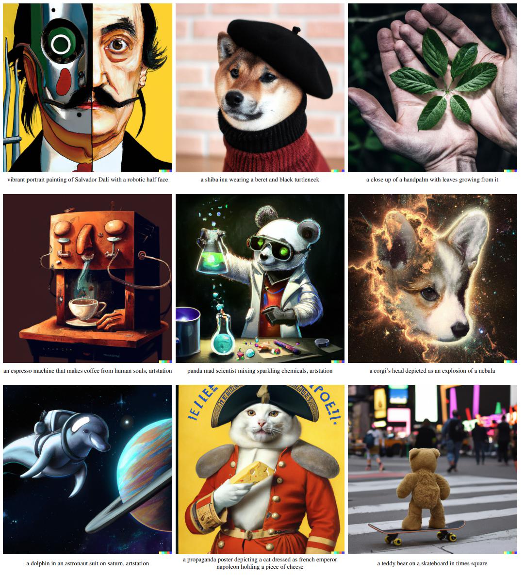
Figure 4. Modification of an input image (right) with a new caption.
Image manipulation
Image variation
Given an input image, the CLIP image encoder gives an embedding \(z_i\) that can be passed back through the decoder to generate variations of this image (thus without caption/CLIP text embedding conditioning). The stochasticity is introduced by the parameter \(\eta\) of the DDIM and as the value of this parameter increase, the variations tell us what information was captured in the CLIP image embedding.

Figure 5. Vatiations of an input image.
Interpolation
Following trajectories between two CLIP latent representations (obtained from two images or two text prompts) allow doing interpolation.
Note : as CLIP space is normalized, the interpolation is done with spherical linear interpolation function slerp.
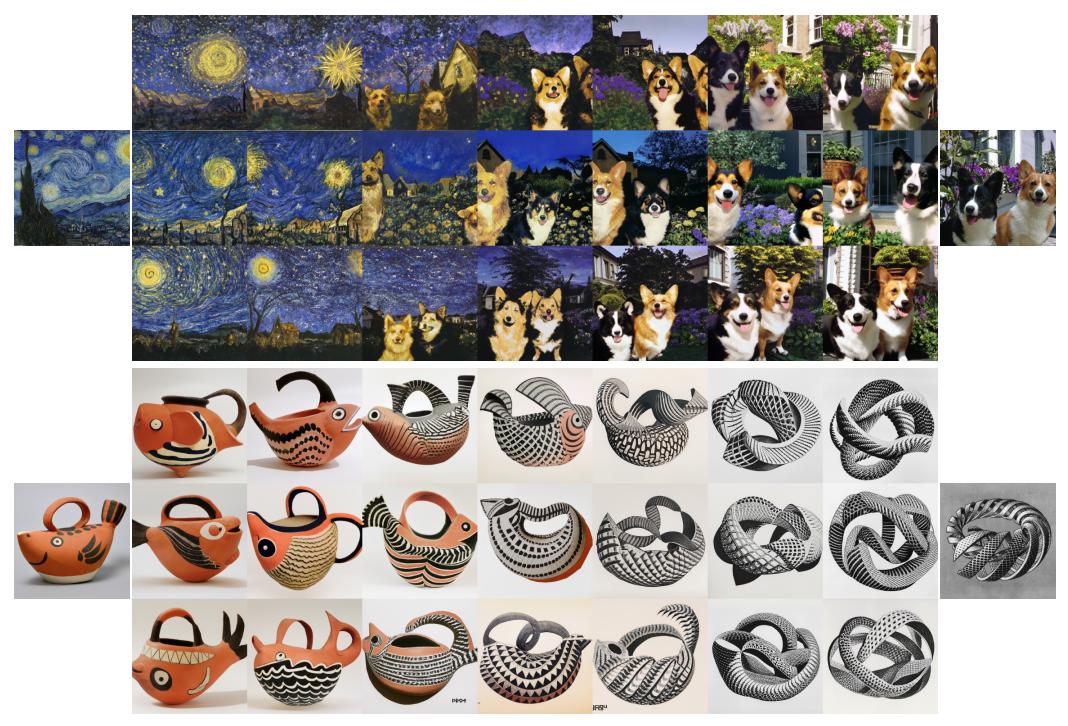
Figure 6. Interpolation between images.
Text diffs
As the texts and images are embedded in the same space, it is possible to do language guided image manipulations such as text diffs. For example, let’s take an image \(x\), caption \(y_0\) describing this image and a new text description \(y\) that we would like to use to modify the image. We can paritally interpolate between the CLIP image embedding \(z_i\) and the text diff vector \(z_d = \text{norm}(z_t - z_{t_0})\) (via \(z_\theta = \text{slerp}(z_i, z_d, \theta)\), with \(\theta\) ranging from 0 to a value generally between 0.25 and 0.5)

Figure 7. Modification of an input image (right) with a new caption.
References
-
See this tutorial on transformers ↩
-
A. Nichol, P. Dhariwal, A. Ramesh, P. Shyam, P. Mishkin, B. McGrew, I. Sutskever, M. Chen, GLIDE: Towards Photorealistic Image Generation and Editing with Text-Guided Diffusion Models ↩
-
J. Song, C. Meng, S. Ermon, Denoising Diffusion Implicit Models, International Conference on Learning Representations (ICLR), 2021. ↩
-
J. Ho, T. Salimans, Classifier-Free Diffusion Guidance, NeurIPS 2021 Workshop on Deep Generative Models and Downstream Applications ↩