OSS-Net: Memory Efficient High Resolution Semantic Segmentation of 3D Medical Data
Notes
- Link to the code here
Highlights
- The goal of the paper is to perform segmentation using neural implicit functions (NIFs) to avoid memory limitations of 3D CNNs.
- The authors build up on Occupancy Networks to include advantages from 3D CNNs and NIFs and apply their method to segmentation of tumors.
Introduction
State-of-the-art in 3D medical data segmentation relies on 3D CNNs that have significant limitations regarding their computation complexity and the memory consumption which grows cubically in memory.
The authors propose to get rid of the voxelized structure and to use NIFs (see previous post 1 for more details) and focus on Occupancy Networks (ONet) 2.
However, ONet is slow at inference and its expressiveness is limited because it uses a global latent code to represent a shape.
Therefore authors combine a 3D CNN encoder with an ONet decoder to take advantage of the segmentation performance of 3D CNNs and the memory efficiency of ONet.
Method
What are Occupancy Networks (ONet)? ONets are networks which learn an occupancy function representing a 3D object. This is described by the mapping: \(f_{\theta}:\mathbb{R}^3 \times \mathcal{X} \rightarrow [0,1]\). The inputs are the coordinates of a point \(p\in\mathbb{R}^3\) and an observation \(x\in\mathcal{X}\). The output is the occupancy probability \(o\in[0,1]\) for the point given the observation. This value \(o\) expresses whether the point \(p\) is located inside (\(o=1\)) or outside (\(o=0\)) of the continuous object boundary.
In OSS-Net, they add a local observation \(z\), which is a local patch around the point. This is thus described by the mapping: \(f_{\theta}:\mathbb{R}^3 \times \mathcal{X} \times \mathcal{Z} \rightarrow [0,1]\).
Architecture
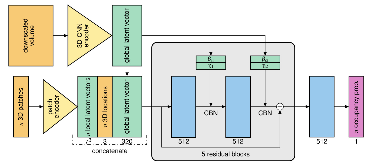
Figure 1: OSS-Net architecture
The architecture of OSS-Net includes:
- a 3D CNN encoder
- ResNet-like architecture
- input: downscale 3D volume \(x\)
- ouput: global latent vector which consists in the concatenation of the output skip connections (see Fig. 2)
- output: a low resolution segmentation (used in an auxiliary loss and during inference to increase speed)
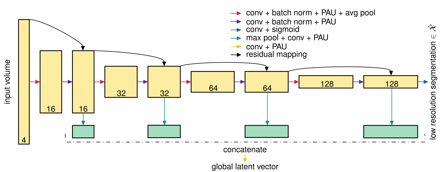 Figure 2: 3D CNN encoder architecture
- a patch encoder
- consists in two 3D convolution layers
- input: \(n\) patches \(z\) corresponding to \(n\) locations \(p\) in the volume
- output: \(n\) local latent vectors (one for each patch)
- an ONet decoder
- fully-connected ResNet architecture
- CBN: Conditional Batch-Normalization with parameters \(\beta\) and \(\gamma\) predicted from the global latent vector
- input: concatenation of global and local latent vector and the \(n\) coordinates
- output: occupancy probability at the \(n\) locations
Loss
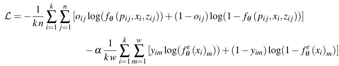 Figure 3: OSS-Net loss
Two terms in the loss:
- a binary cross-entropy between the reference occupancy probability \(o_{ij}\) of the sampled points and the predicted occupancy probability \(f_\theta(p_{ij},x_i,z_{ij})\)
- an auxiliary loss: also a binary cross-entropy between the reference label value \(y_{im}\) and the predicted low resolution segmentation label \(f_\theta^\mathcal{e}(x_i)_m\) (output of the 3D CNN encoder)
Notation:
- \(k\) is the size of the mini-batch
- \(n\) is the number of sampled points
- \(w\) is the total number of voxels
- \(\alpha\) is a weighting factor, set to 0.1
Inference: MISE algorithm
The MISE (Multiresolution IsoSurface Extraction) algorithm (also from the original ONet paper 2) is used to extract the predicted decision boundary of the OSS-Net. With this algorithm, they can produce an accurate segmentation while reducing the inference time.
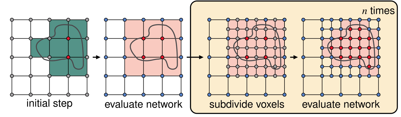 Figure 4: 2D visualization of the MISE algorithm in OSS-Net
Original MISE algorithm steps:
- discretization of the space at initial resolution
- evaluation for all the points in the grid
- voxels with at least two adjacent grid points with different prediction marked as active (in pink in the Fig. 4)
- subdivision of the active voxels
- Repeat step 2 to 4 until final resolution is reached
For OSS-Net, the authors also use the low resolution segmentation map as an initial state, which replaces the first evaluation step. This results enables a faster inference because less locations have to be queried to reach the desired resolution.
Datasets
BraTS 2020
- MRI brain images
- brain tumor segmentation: OSS-Net : merge all labels in one
- publicly available volume + reference: 320/45 for train/val
LiTS
- abdominal CT scans
- liver tumor segmentation: OSS-Net: full liver segmentation (tumor + liver merged in one)
- publicly available volume + reference: 111/20 for train/val
- downscaled to fit in GPU
Data augmentation: flipping, brightness adjustment, gaussian noise injection
Results
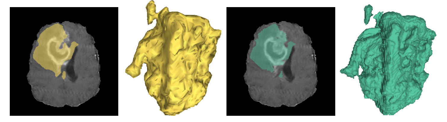 Figure 5: Brain tumor segmentation results (left:predicted, right:reference)
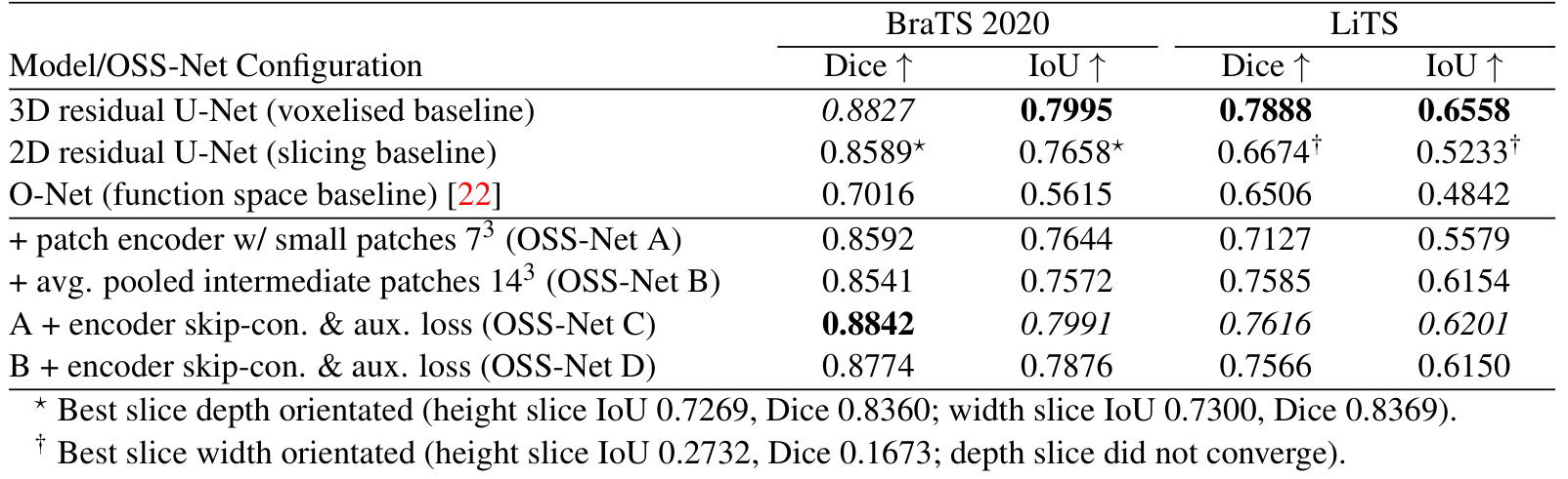 Table 1: Segmentation results for OSS-Net and baselines
Comparison with baselines:
- Better than function space baseline (ONet),
- For BraTS, on par with voxelised baselines (3D residual UNet)
- For LiTS, slightly lower than voxelised baseline, maybe due to smaller dataset
Comparison of proposed models:
- improvements from the 3D CNN encoder (C and D)
- increase of patch size does not bring better results
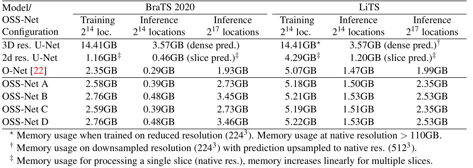 Table 2: GPU memory consumption of OSS-Net and baselines
Comparison with baselines:
- more memory efficient than voxelised baselines (3D residual UNet) in training and inference
- slightly not as efficient as ONet during inference
- not as efficient as slicing baseline (2D residual UNet) in training and on par for inference
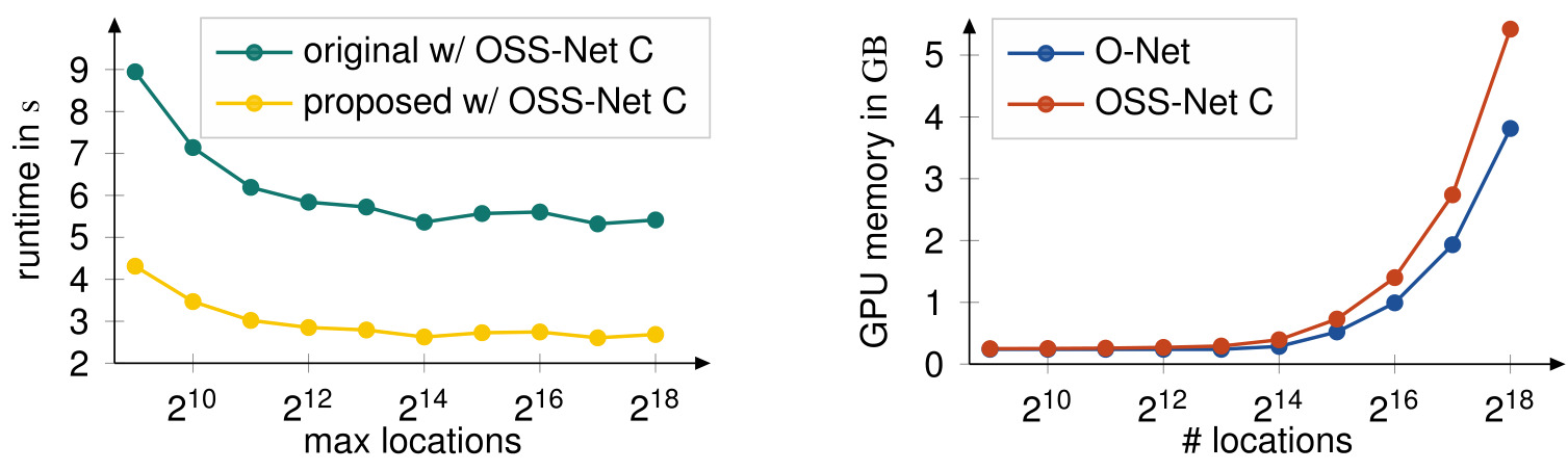 Figure 6: Inference runtime (left) and memory performance (right) of OSS-Net
Proposed approach is the inference based on the low-resolution segmentation. It is two times faster for inference whatever the number of points used.
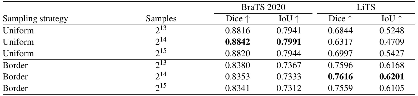 Table 3: Comparison of different sampling strategies
“Uniform”: random sampling
“Border”: sampling more densely near the border of the regions of interest
Conclusion
The advantages os OSS-Net as shown here are:
- compared to the original function space (ONet)
- the use of local observation as input produces finer structures,
- better inference speed due to the 3D CNN encoder
- compared to a full 3D CNN baseline
- on par results but smaller memory cost
The authors also suggest that the last layer could be adapted to multi-structure segmentation.