Multi-modal Variational Autoencoders for normative modelling across multiple imaging modalities

Notes

Link to Tutorial VAE

No Github repository.

Figures to help understand examples of Multi-modal VAE, one with a Product of Experts loss and the other with a Mixture of Experts loss.

• Multi-modal VAE (Product of Experts loss):

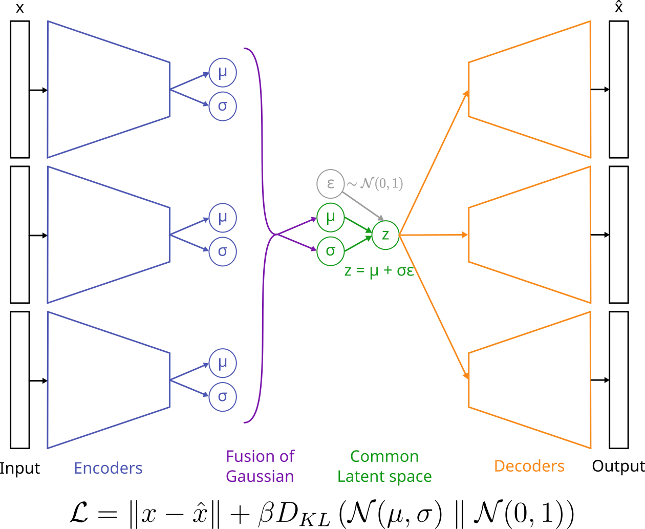Figure adapted from A. Salvador

• Multi-modal VAE (Mixture of Experts loss):

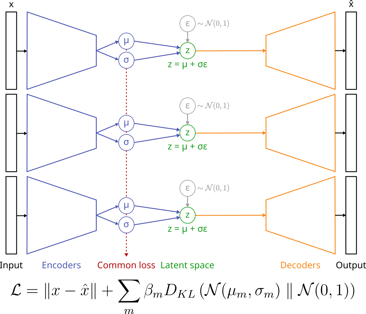Figure adapted from A. Salvador

 

Highlights

In this paper, the authors introduce two contributions:

• They present two multi-modal normative modelling frameworks (MoE-normVAE, gPoE-normVAE).
• They use a deviation metric that is based on the latent space.

 

Introduction

• Authors study heterogeneous brain disorders and use normative models. These models assume that disease cohorts are located at the extremes of the healthy population distribution.

• However, it is often unclear which imaging modality will be the most sensitive in detecting deviations from the norm caused by brain disorders. Hence, they choose to develop normative models that are suitable for multiple modalities.

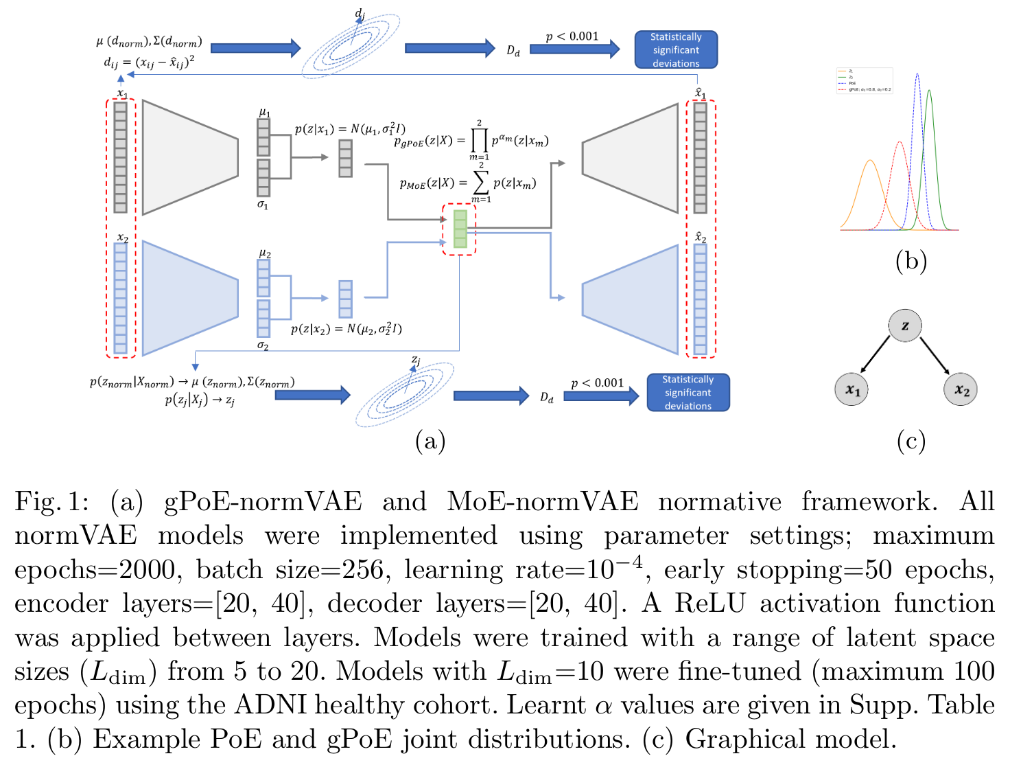
• Multi-modal VAE frameworks usually learn separate encoder and decoder networks for each modality and aggregate the encoding distributions to learn a joint latent representation (cf. figure in Notes). One approach is the Product of Expert (PoE) method, which considers all experts to be equally credible and assigns a uniform contribution from each modality. Nevertheless the joint distribution can be biased due to overconfident experts.

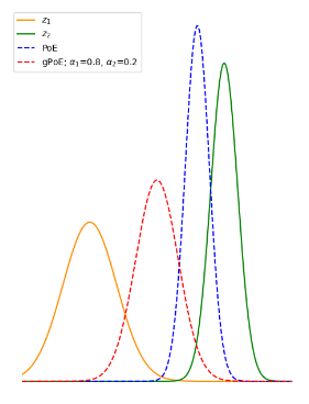
Fig 1. (b) Example PoE and gPoE joint distributions.

• Authors propose a generalised Product-of-Experts (gPoE) by adding a weight to each modality and each latent dimension. They also use the Mixture of Expert (MoE) model and compare it with other methods.

• Finally, to exploit this joint latent space, they develop a deviation metric from the latent space instead of the feature space.

 

Method

Product of Experts

• $M$ : number of modalities

• $\pmb{X} = \left \{ {\pmb{x}_m} \right \}_{m=1}^{M}$ : Observations

• $p(\textbf{z})$ : prior

• $p_{\theta}(\pmb{X}, \pmb{z}) = p(\pmb{z})\prod_{m=1}^{M} p_{\theta_{m}}(\pmb{x}_m \vert \pmb{z})$ : likelihood distribution
• $\theta = \left \{ \theta_{1},...,\theta_{M} \right \}$ : Decoder parameters

$$\mathcal{L} = \mathbb{E}_{q_{\phi}(\pmb{z} \vert \pmb{X})}\left[\sum_{m=1}^{M} log \ p_{\theta}(\pmb{x}_m \vert \pmb{z})\right] - D_{KL}\left( q_{\phi}(\pmb{z} \vert \pmb{X}) \parallel p(\pmb{z})\right)$$

• $q_{\phi}(\pmb{z} \vert \pmb{X}) = \frac{1}{K} \prod_{m=1}^{M} q_{\phi_{m}}(\pmb{z} \vert \pmb{x}_m)$ : probability density function
• $\phi = \left \{ \phi_{1},...,\phi_{M} \right \}$ : Encoder parameters

They assume that each encoder follows a gaussian distribution:

$$q(\pmb{z} \vert \pmb{x}_m) = \mathcal{N} (\pmb{\mu}_m, \pmb{\sigma}_{m}^{2}\pmb{I})$$

Therefore,

$$\pmb{\mu} = \frac{\sum_{m=1}^{M} \pmb{\mu}_m/\pmb{\sigma}_{m}^{2}}{\sum_{m=1}^{M} 1/\pmb{\sigma}_{m}^{2}}$$ $$\pmb{\sigma}^{2} = \frac{1}{\sum_{m=1}^{M} 1/\pmb{\sigma}_{m}^{2}}$$

 

Mixture of Experts

In the case of MoE, the probability density function becomes:

$$q_{\phi}(\pmb{z} \vert \pmb{X}) = \frac{1}{K} \sum_{m=1}^{M} \frac{1}{M} q_{\phi_{m}}(\pmb{z} \vert \pmb{x}_m)$$

and the loss:

$$\mathcal{L} = \sum_{m=1}^{M} \left [ \mathbb{E}_{q_{\phi}(\pmb{z} \vert \pmb{X})}\left[\sum_{m=1}^{M} log \ p_{\theta}(\pmb{x}_m \vert \pmb{z})\right] - D_{KL}\left( q_{\phi}(\pmb{z} \vert \pmb{x}_m) \parallel p(\pmb{z})\right) \right ]$$

• Disadvantage: the model only considers each uni-modal encoding distribution independently and does not explicitly combine information from multiple modalities in the latent representations.

 

Generalised Product-of-Experts joint posterior

To overcome the problem of overconfident experts, they added a weighted term for each modality and each latent dimension on the joint posterior distribution.

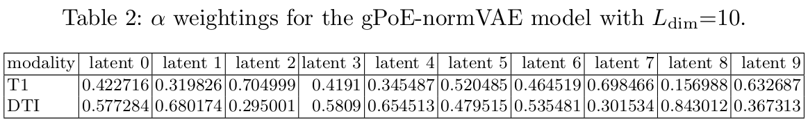
$$q_{\phi}(\pmb{z} \vert \pmb{X}) = \frac{1}{K} \prod_{m=1}^{M} \frac{1}{M} q_{\phi_{m}}^{\alpha_{m}}(\pmb{z} \vert \pmb{x}_m)$$

With: $\sum_{m=1}^{M} \alpha_{m}=1$ and $0 < \alpha_{m} < 1$ ($\alpha$ is learned during training)

Exemple of $\alpha$:

Just like the PoE approach, the parameters of the joint posterior distribution can be calculated:

$$\pmb{\mu} = \frac{\sum_{m=1}^{M} \pmb{\mu}_m\pmb{\alpha}_m/\pmb{\sigma}_{m}^{2}}{\sum_{m=1}^{M} \pmb{\alpha}_m/\pmb{\sigma}_{m}^{2}}$$ $$\pmb{\sigma}^{2} = \frac{1}{\sum_{m=1}^{M} \pmb{\alpha}_m/\pmb{\sigma}_{m}^{2}}$$

 

Multi-modal latent deviation metric

• Previous work used the following distance (a univariate feature space metric) to highlight subjects that are out of distribution:

$$D_{uf} = \frac{d_{ij} - \mu_{norm}(d_{ij}^{norm})}{\sigma_{norm}(d_{ij}^{norm})}$$

$\mu_{norm}(d_{ij}^{norm})$ and $\sigma_{norm}(d_{ij}^{norm})$ represent the mean and standard deviation of the holdout healthy control cohort.

• The authors suggest that using latent space deviation metrics would more accurately capture deviations from normative behavior across multiple modalities. They measure the Mahalanobis distance from the encoding distribution of the training cohort:

$$D_{ml} = \sqrt{(z_j - \mu(z^{norm}))^T \ \Sigma(z^{norm})^{-1} \ (z_j - \mu(z^{norm})) }$$

where $z_j \sim q(\pmb{z}_j \vert \pmb{X}_j)$ is a sample from the joint posterior distribution for subject $j$, $\mu(z^{norm})$ and $\Sigma(z^{norm})$ are respectively the mean and the covariance of the healthy control cohort latent position.

• Finally, for closer comparaison with $D_{ml}$, they derive it to the multivariate feature space:

$$D_{mf} = \sqrt{(d_j - \mu(d^{norm}))^T \ \Sigma(d^{norm})^{-1} \ (d_j - \mu(d^{norm})) }$$

where $d_j = \left \{ d_{ij},...d_{Ij}\right \}$ is the reconstruction error for subject $j$ for brain regions $(i = 1, ..., I)$.

 

Assessing deviation metric performance

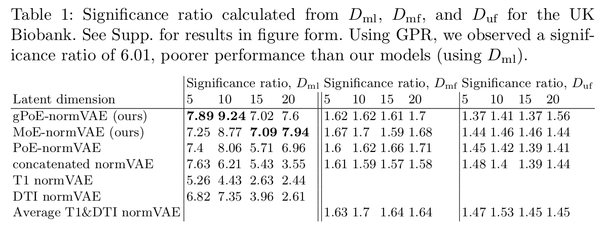
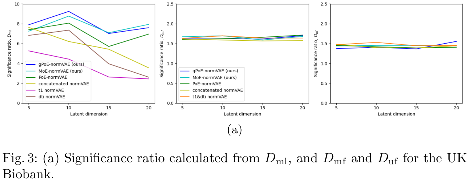
To evaluate the performance of their models, they use the significance ratio:

$$significance \ ratio = \frac{True \ positive \ rate}{False \ positive \ rate} = \frac{\frac{N_{disease}(outliers)}{N_{disease}}}{\frac{N_{holdout}(outliers)}{N_{holdout}}}$$

Ideally, we want a model which correctly identifies pathological individuals as outliers and healthy individuals as sitting within the normative distribution.

 

Architecture

• Dataset used: UK Biobank
• 10,276 healthy subject to train their neural networks
• At test time:
  • 2,568 healty controls from holdout cohort
  • 122 individuals with one of several neurodegenerative disorders
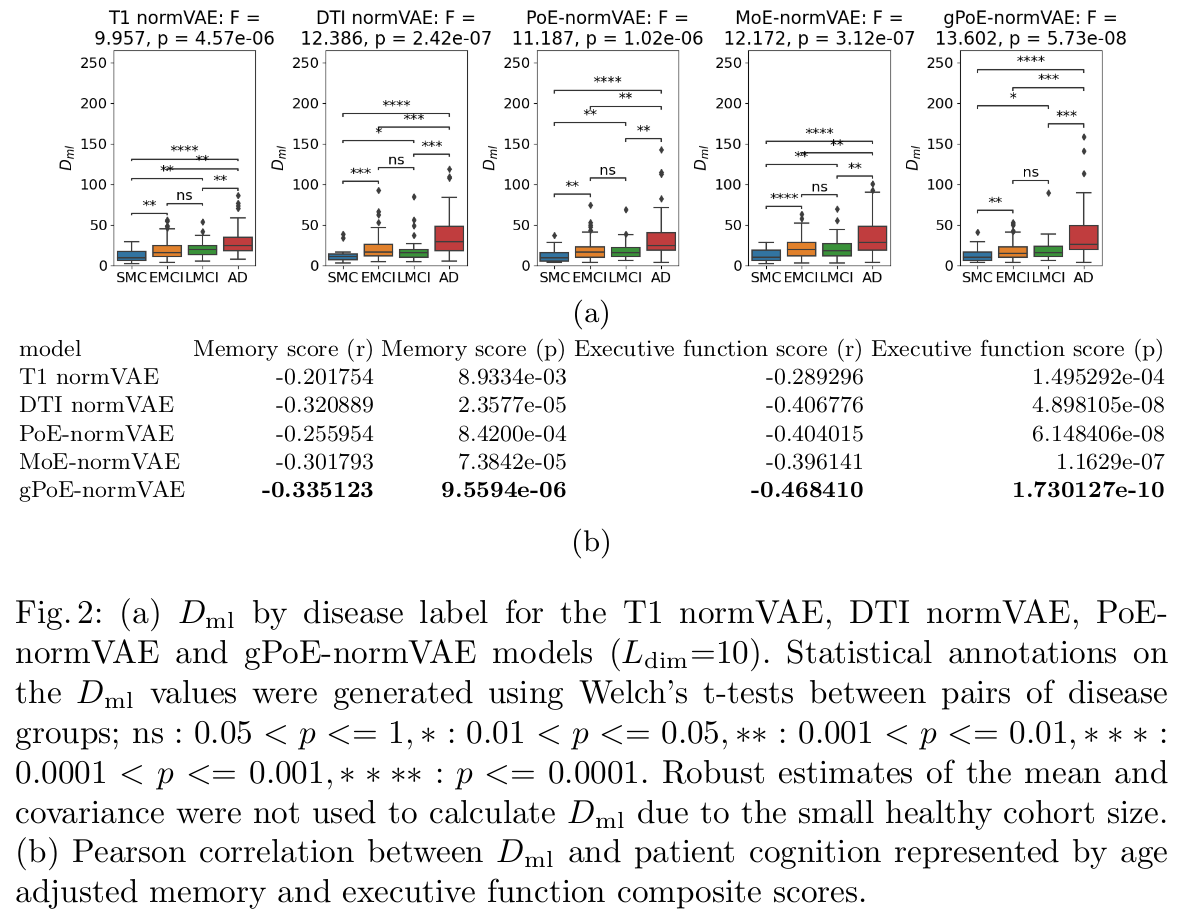
• Also tried on another dataset: Alzheimer’s Disease Neuroimaging Initiative (ADNI) with 213 subjects
• (same image modality were extracted (T1 and DTI features) for both datasets)

 

Results

For the UK Biobank dataset:

For the ADNI dataset:

 

Conclusions

• Their models provide a better joint representation compared to baseline methods.
• They proposed a latent deviation metric to detect deviations in the multivariate latent space.