Tracking Everything Everywhere All at Once
Notes
Project page: https://omnimotion.github.io/
Github: https://github.com/qianqianwang68/omnimotion
Introduction
Method to estimate long-range motion (point tracking) in a video by learning a canonical representation of the motion given noisy estimates. This method is a test-time optimization method as it does not train on a dataset containing multiple samples but rather performs optimization at test-time on a single sample.
Preliminaries
This work is built upon various methods.
Neural implicit representation
A neural implicit representation describes a signal (like a 3D shape, image, or motion field) as a continuous function learned by a neural network, rather than as discrete pixels or voxels. Given a coordinate (e.g., position or time), the network outputs the corresponding value (like color, density, or displacement), allowing smooth, resolution-independent reconstruction.
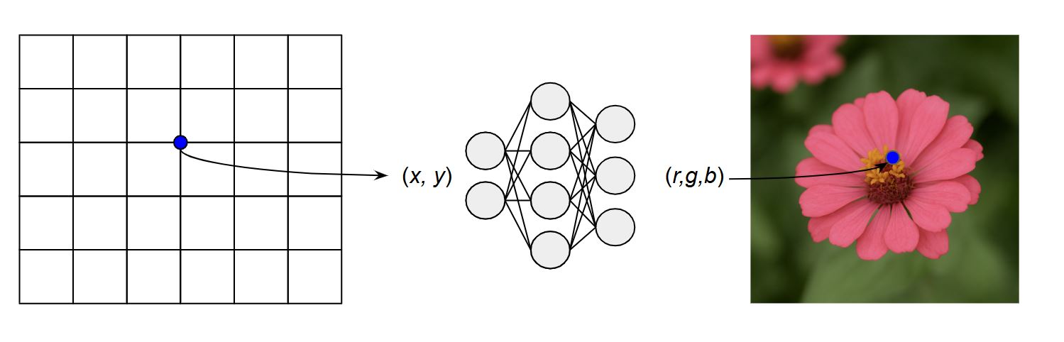
Figure 1. Example of a simple neural implicit representation.
NeRF (Neural Radiance Fields)
NerF is a model that learns a continuous 3D scene representation by mapping 3D coordinates and viewing directions to color and density using a neural network1.
By integrating these values along camera rays, NeRF can render realistic novel views of a scene from any angle.
See https://creatis-myriad.github.io/2023/01/31/NeRF.html for more details.
Invertible neural networks
An invertible neural network (INN) is a model where every layer is designed to be mathematically reversible, so inputs can be exactly recovered from outputs. The network can therefore learn a bijective mapping between spaces.
This is usually done by stacking multiple couple layers. Each coupling layer separates its input into two. The first input is used to generate the parameters of a simple transform (ex., scaling and addition) which is applied to the second input while the first input is preserved. The generation of the transformation parameters can be done with a complex function (neural network). To make an invertible neural network, multiple coupling layers are stacked, alternating which input is preserved and which is transformed.
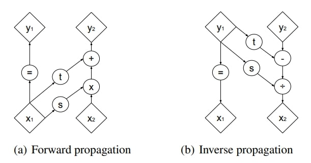
Figure 2. Example of an invertible layer. Figure from 2
Method
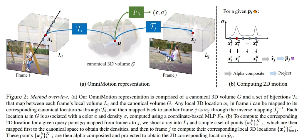
Figure 3. Method overview.
Canonical representation
The goal of the method is to learn a 3D canonical volume \(G\) that represents the motion. In this volume, points \(u\) represent a time-independent representation of the point in the image space.
To map a 3D point \(x_i\) in frame \(i\) to its 3D canonical coordinate \(u\), a bijective mapping \(\mathcal{T}_i\) is used. This allows the mapping of a point \(x_i\) in frame \(i\) to be mapped to a point \(x_j\) in frame \(j\) with the inverse mapping:
\[x_j = \mathcal{T}^{-1}_j \circ \mathcal{T}_i(x_i)\]The bijective function \(\mathcal{T}\) is implemented with an invertible neural network (Real-NVP2). The conditioning on the time index is done with a frame latent code \(\psi_i\) such that one neural network can parametrize all the bijections: \(\mathcal{T}_i(\cdot) = M_\theta(\cdot;\psi_i)\). The latent code is computed with a separate MLP.
The following figure shows one layer (of six) of the invertible neural network used in the paper.
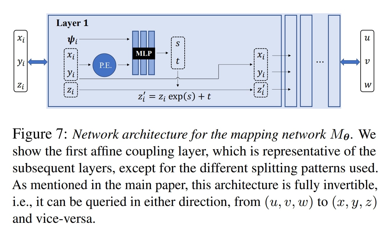
Figure 4. Illustration of one of the layers in the invertible mapping function.
Frame to frame 2D motion
To compute the motion of a 2D point (i.e., its position in another frame), it is first “lifted” into 3D by sampling along a ray. The 3D point is mapped into the canonical volume and unmapped back to a different frame, where it is projected back to 2D.
More formally, this can be broken down into the following steps:
1. 2D to 3D ray tracing.
For a fixed, orthographic camera and a given 2D point \(p_i\) in frame \(i\), 3D points are samples at multiple depths \(\{z_i^k\}_{k=1}^K\) are sampled along a ray \(r_i(z) = \mathbf{o}_i + z\mathbf{d}\), where \(\mathbf{o}_i = [p_i, 0]\) and \(\mathbf{d}=[0,0,1]\). The output is a set of 3D points: \(\{x_i^k\}_{k=1}^K\).
2. Mapping to canonical space
Each point \(x_i^k\) is mapped to the canonical space \(u^k = \mathcal{T}_i(x_i^k) = M_\theta(x_i^k; \psi_i)\).
3. NeRF color and density prediction
Like in NeRF, the densities and colors of each of these canonical points \(\{u^k\}\) are computed: \((\sigma_k, \mathbf{c}_k) = F_\theta(u^k)\). \(F_\theta\) is a MLP implemented as a Gabor network 3.
4. Inverse mapping
Each point \(u^k\) is mapped back to 3D space at frame \(j\): \(x_j^k = \mathcal{T}^{-1}_j(u^k)= M^{-1}_\theta(u^k; \psi_j)\).
5. Alpha compositing: point and color
To find a single 3D point prediction in frame \(j\), alpha compositing is used on all the points \(x^k_j\):
\[\hat{x}_j = \sum_{k=1}^K T_k \alpha_k x_k^j , \quad \text{where} \quad T_k = \prod_{l=1}^{k-1}(1 - \alpha_l),\]where \(\alpha_k = 1 - \text{exp}(-\sigma_k)\).
The same is done to get a color prediction \(\hat{\mathbf{C}}_i\) for the point.
6. 2D projection
Given the predicted 3D point \(\hat{x}_j\), the predicted pixel location \(\hat{p}_j\) can be computed by projecting the point with the assumed camera parameters.
Optimization
The optimization process is done for each video. The input for the optimization is the video and a set of filtered pairwise noisy correspondence predictions obtained from another method (ex., RAFT).
The total loss function is a sum of three losses. The first is the flow loss between the predicted flow and the input flow:
\[\mathcal{L}_{flo} = \sum_{\mathbf{f}_{i \rightarrow j} \in \Omega_f} ||\hat{\mathbf{f}}_{i \rightarrow j} - \mathbf{f}_{i \rightarrow j} ||_1,\]where \(\Omega_f\) is the set of input flow pairs. The second is the photometric loss (like NeRF):
\[\mathcal{L}_{pho} = \sum_{(i,\mathbf{p}) \in \Omega_p} ||\hat{\mathbf{C}}_i(p) - \mathbf{C}_i(p) ||^2_2,\]where \(\Omega_p\) is the set of all pixel locations over all frames. Finally a regularization term to penalize large accelerations is added between consecutive triplets of 3D points.
\[\mathcal{L}_{reg} = \sum_{(i,\mathbf{x}) \in \Omega_x} ||\mathbf{x}_{i+1} + \mathbf{x}_{i-1} - \mathbf{x}_i ||_1,\]where \(\Omega_x\) is the union of local 3D spaces for all frames. The final loss function is given by :
\[\mathcal{L} = \lambda_{flo}\mathcal{L}_{flo} + \lambda_{pho}\mathcal{L}_{pho} + \lambda_{reg}\mathcal{L}_{reg}\]The loss weights are given by a scheduler detailed in the supplementary materials.
Hard-mining sampling
Using all pairwise optical flows gives the model lots of motion information, but most of it comes from static background areas that are easy to match. Moving or deforming objects have fewer reliable matches, so the model tends to ignore them. To fix this, the authors track where the model’s flow predictions are most wrong and sample those difficult regions more often during training.
Results
The results show that the method performs well on TAP-Vid benchmark 4. The most important metric, \(<\delta_{avg}^x\), measures how accurately predicted points match their ground truth positions, averaged over five pixel-distance thresholds (1, 2, 4, 8, 16).
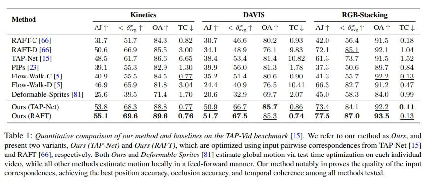
Table 1. Comparison with state-of-the-art methods.
The authors perform an ablation study with some important parameters:
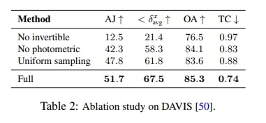
Table 2. Ablation study.
Limitations
- The method struggles with rapid and highly non-rigid motion.
- The method is sensitive to initialization
- The method requires a long optimization for each video (8~9h on an A100 GPU and 12-13h on RTX4090)
Improvements
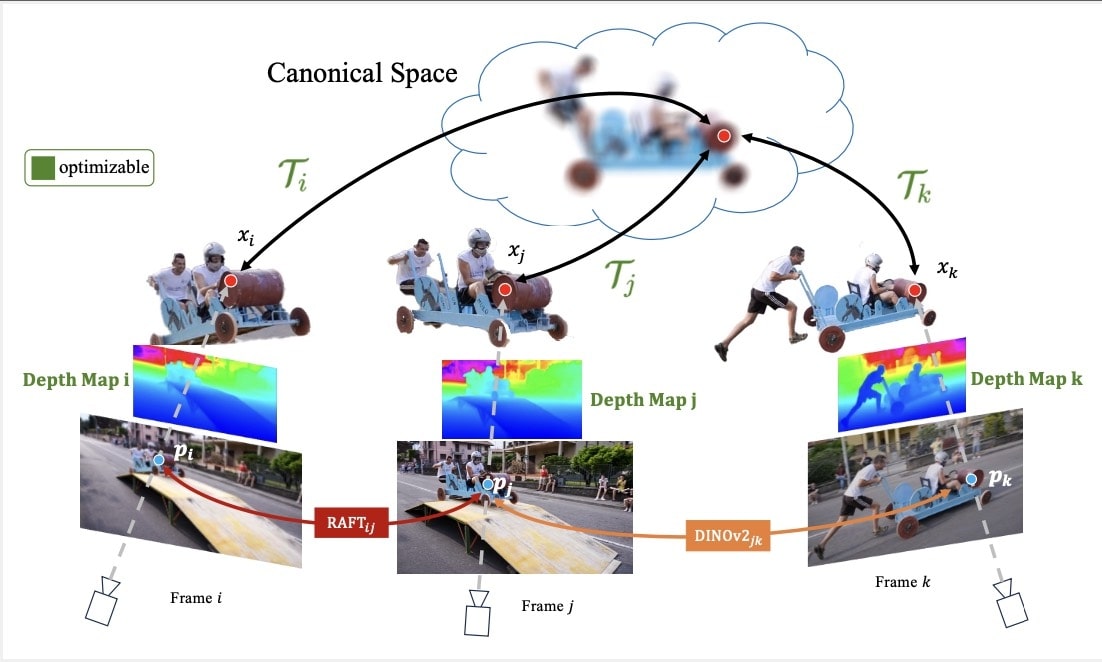
Figure 5. Overview of Track Everything Everywhere Fast and Robustly.
An improved version of this method was presented at ECCV 2024: Track Everything Everywhere Fast and Robustly 5. They propose three key improvements:
- The NeRF-like photometric loss is removed, and the depth estimation is replaced with a pre-trained depth estimation method (ZoeDepth).
- A new and more expressive invertible neural network is proposed.
- In addition to RAFT, DinoV2 is used to generate more long-term noisy estimates for the motion.
This improvement greatly improves the robustness to initialization and optimization speed.
References
-
Mildenhall et al.. NeRF: Representing Scenes as Neural Radiance Fields for View Synthesis. ECCV 2020. ↩
-
Dinh et al.. Density estimation using Real NVP. ICLR 2017. ↩ ↩2
-
Fathony et al.. Multiplicative filter networks. ICLR 2021. ↩
-
Doersch et al.. TAP-Vid: A Benchmark for Tracking Any Point in a Video. Neurips 2022. ↩
-
Song et al.. Track Everything Everywhere Fast and Robustly. ECCV 2024. ↩