Notes

Link to the code here
This post is strongly linked with the Bayesian inference tutorial

Motivations

Deep learning methods have traditionally struggled with tabular data, because of the heterogeneity between datasets and the heterogeneity of the raw data itself.
Tables contain columns, also called features, with various scales and types (Boolean, categorical, ordinal, integer, floating point), imbalanced or missing data, unimportant features, outliers and so on.
This made non-deep-learning methods, such as tree-based models, the strongest contender so far.

Highlights

Introduction of a foundation model for small to medium-sized tabular data
Efficient supervised tabular learning method for any small to moderate-sized dataset
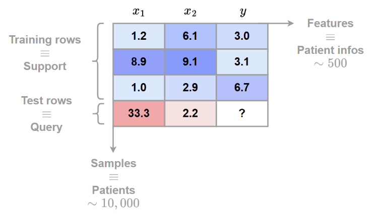
Yields among the best performance for datasets with up to 10,000 samples (lines) and 500 features (columns).
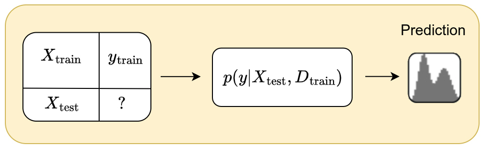
Based on in- context learning:
\[p(y_{\text{test}} \mid X_{\text{test}}, D_{\text{train}})\]
where \(D_{\text{train}} = (X_{\text{train}}, y_{\text{train}})\)

Mathematical concepts

A complete demonstration can be found in the Bayesian inference tutorial

TabPFN is based on the amortized simulation-based inference formalism, whose aim is to model the ouput \(y\) from a new input \(x\) based on a supervised dataset \(D=(X_{\text{train}},y_{\text{train}})\) of arbitrary size \(n\).
The goal is therefore to model the posterior predictive distribution \(p(y \mid x, D)\). Since we explicitly use a support dataset \(D\) to predict \(y\) from \(x\), this model falls under in-context learning.

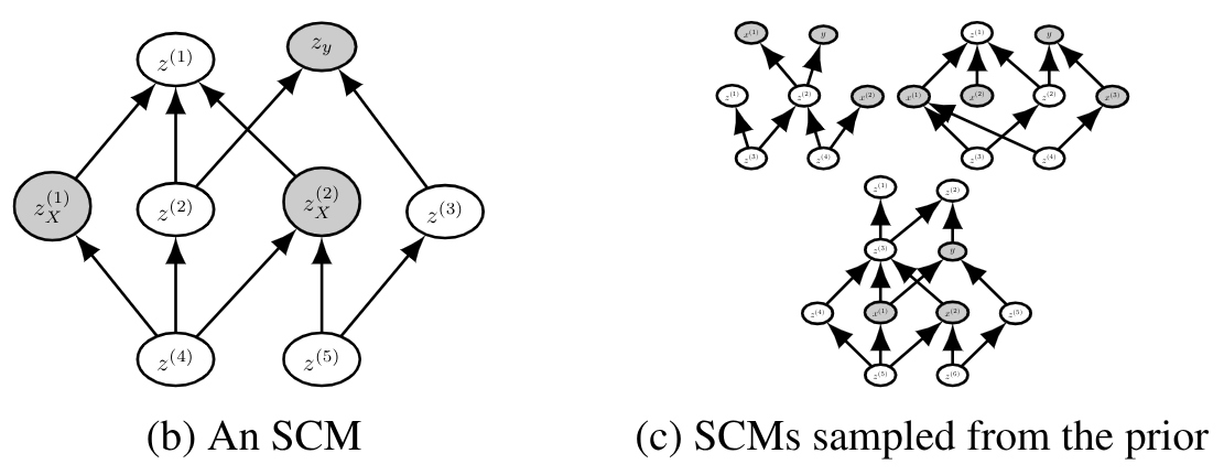
Prior modeling through Structural Causal Models (SCMs)

Tabular data can be seen as the result of several simple mechanisms interacting with each other.

a table row corresponds to a real-world entity (patient, customer, transaction, etc.)
each column corresponds to a measurement, decision, or attribute produced by a real process
the label represents a consequence (diagnosis, defect, class, etc.)

Tabular data result from chains of decisions, mechanisms, and constraints. Even if the exact causal structure is unknown, tabular data are almost always causal in essence.

Causality refers to the fact that variables are linked through cause–effect relationships, even if their exact structure is unknown.

Structural Causal Models (SCMs) are thus used as the prior to model the implicit structure of tabular data. They impose a “reasonable” structure without being rigid.

They model:

nonlinear dependencies
interactions
noise
different graphs (i.e. relationships) across datasets

They allows:

local, compositional, and parsimonious structures
plausible dependencies between columns
preference for simple relationships

Synthetic dataset generation

To generate a synthetic dataset, TabPFN essentially follows the following pipeline:

Sample a causal structure (DAG)
Sample the causal mechanisms
Sample noise terms
Generate the features
Generate the label
Apply realistic transformations
Sample a small dataset (few-shot regime)

Each dataset corresponds to a task for which TabPFN learns to perform Bayesian inference.

1- Sample a causal structure (DAG)

Number of variables: randomly sampled within a range (e.g., 5 to 100)
Graph structure
- sparsity is encouraged
- a small number of parents per node
- a random topological ordering

The intuition beind this sampling scheme is that real-world tabular variables rarely exhibit global dependencies across all columns

2- Sample the causal mechanisms

The following relation is defined for each variable \(X_i\) with parents \(Pa(X_i)\): \(X_i = f_i \left( Pa(X_i) \right) + \epsilon_i\)

\(f_i\) is randomly chosen from a mixture of function families:

linear functions
simple nonlinear functions
small neural networks
sometimes tree- or threshold-based function

But with:

low depth
low complexity
simple activations

3- Sample noise terms

Each variable has its own noise term \(\epsilon_i \sim N(0,\sigma_i^2)\). The variance \(\sigma_i\) is sampled randomly.

4- Generate the features (propagation through the DAG)

Once we have:

the graph
the structural functions
the noise terms,

data are generated according to the causal ordering:

variables without parents \(\rightarrow\) sampled directly
intermediate variables \(\rightarrow\) computed via \(𝑓_i\)
deeper variables \(\rightarrow\) accumulate dependencies and noise

A set of features are then randomly selected from the graph

5- Generate the label \(y\)

The label is treated as a final causal variable.

A value of \(y\) is first randomly selected from the graph and then updated according to the following equation:

\[y = g \left( Pa(y) \right) + \epsilon_y\]

where:

\(g\) is sampled as a simple function
\(y\) sometimes depends on few variables
\(y\) sometimes depends indirectly on many through the DAG

For classification:

\(g\) produces a latent score
passed through a sigmoid or softmax
then the class is sampled

The figure below shows an example of SCMs sampled from the prior. The grey nodes correspond to the sampled inputs \(X\) and output \(y\).

6- Apply realistic transformations

Before feeding the dataset to the model, TabPFN applies:

random normalization
column permutation
different scalings per feature
monotonic transformations
introduction of class imbalance

These steps prevent the model from “cheating” by recognizing the generator.

7- Sample a small dataset (few-shot regime)

Finally:

a small number of samples \(𝑛\) is drawn (often \(<1000\))
train/test split is created
everything is provided in-context to the transformer

Methodology

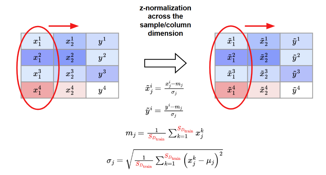
Data preprocessing

Both the synthetic and the real datasets are represented as follows:

The categorical data are encoded as integers

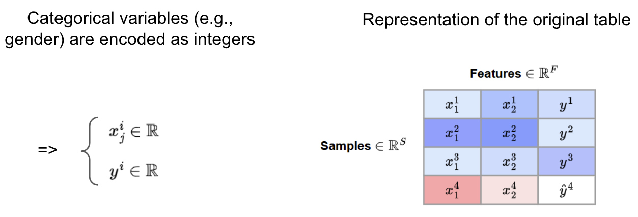
A z-normalization across feature/column dimension is applied

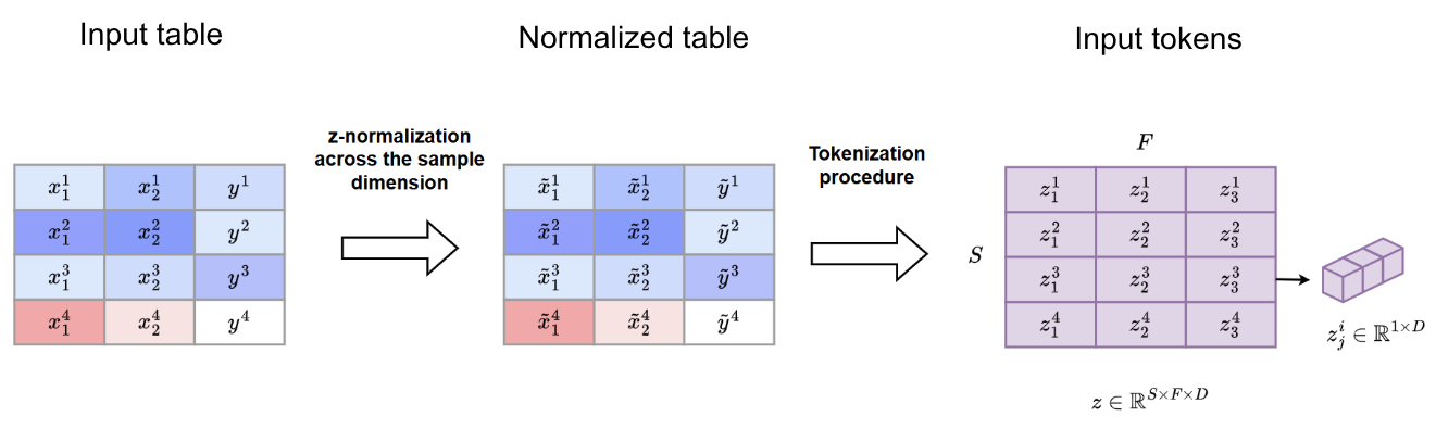
Tokenization procedure

After data preprocessing, each tabular feature is embedded as a token using a shared linear projection

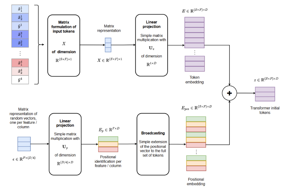
This yields the following representation at the input of the transformer

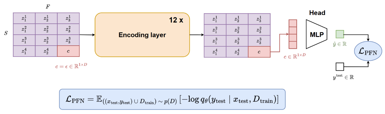
Transformer architecture

The following transformer architecture is proposed. It consists of 12 layers that sequentially apply attention over features and attention over samples. It should be noted that attention over samples is applied between all support samples and one query sample at a time. Query samples do not interact with one another.

Training procedure

During training, each batch is populated with a dataset sampled from the SCM distribution described above. The following scheme is then applied

Implementation

TabPFN was trained for approximately 2,000,000 steps with a batch size of 64 datasets
That means TabPFN is trained on around 130,000,000 synthetically generated datasets !
One training run requires around 2 weeks on one node with eight Nvidia RTX 2080 Ti GPUs
The number of training samples was sampled for each dataset uniformly up to 2,048 and use a fixed validation set size of 128
The number of features was sampled using a beta distribution that was linearly scaled to the range 1–160
To avoid peaks in memory usage, the total size of each table was restricted to be below 75,000 cells by decreasing the number of samples for large numbers of features

Experiments

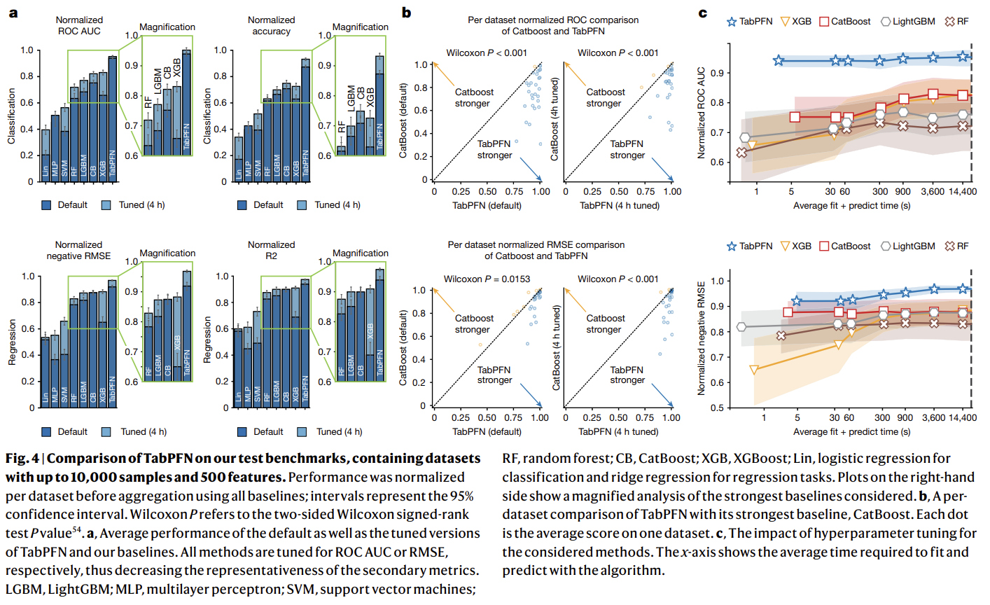
TabPFN was compared against state-of-the-art baselines, including tree-based methods (random forest, XGBoost (XGB), CatBoost, LightGBM), linear models, support vector machines (SVMs) and MLPs
TabPFN was evaluated on two dataset collections: AutoML Benchmark and OpenML-CTR23. These benchmarks comprise diverse real-world tabular datasets, curated for complexity, relevance and domain diversity
From these benchmarks, the authors used 29 classification datasets and 28 regression datasets that have up to 10,000 samples, 500 features and 10 classes
Evaluation metrics include ROC AUC and accuracy for classification, and R2 and negative RMSE for regression
Scores were normalized per dataset, with 1.0 representing the best and 0.0 the worst performance with respect to all baselines
Hyperparameters were tuned using random search with five-fold cross-validation, with time budgets ranging from 30 s to 4 h
All methods were evaluated in inference using eight CPU cores, with TabPFN additionally using one GPU (RTX 2080 Ti)

Results

1- Comparison with state-of-the-art baselines

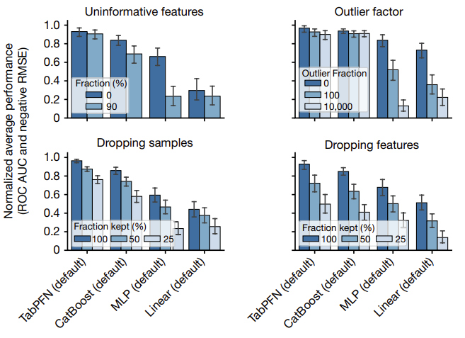
2- Evaluating diverse data attributes

The figure below provides an analysis of the performance of TabPFN across various dataset types:

add uninformative features (randomly shuffled features from the original dataset)
add outliers (multiply each cell with 2% probability with a random number between 0 and the outlier factor)
remove/drop samples
remove/drop features

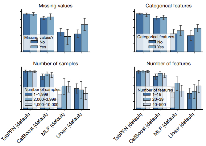
The figure below provides an analysis of the performance of TabPFN on different subgroups:

presence of missing values
presence of categorical features
number of samples
number of features

Conclusions

tabPFN is trained exclusively on synthetic datasets to learn causal structures.
The model was trained on around 130,000,000 synthetically generated datasets !
It can then be efficiently applied at inference time within an in-context framework to classify real-world tabular data without fine-tuning.