Introduction to Bayesian inference
Summary
Introduction
What is a Bayesian method?
A Bayesian method is a statistical approach that relies on Bayes’ theorem to reason under uncertainty.
Main idea
In the Bayesian framework, inference does not reduce to the estimation of a single unknown quantity; rather, uncertainty is encoded via probability distributions and updated as new observations become available.
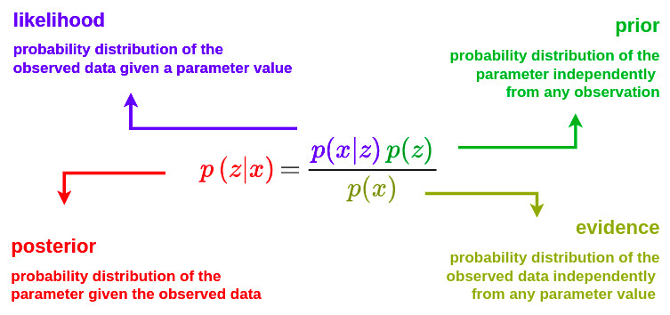
The three key building blocks are:
- The prior probability (prior): what we believe before seeing the data (prior knowledge, assumptions, domain expertise)
- The likelihood: how compatible the observed data are with a given hypothesis
- The posterior probability (posterior): what we believe after seeing the data
A Bayesian method updates probabilistic beliefs based on observed data
What this changes compared to “classical” methods:
- We obtain a full distribution over the parameters (not just a point estimate)
- Uncertainty can be quantified in a natural way
- Prior knowledge can be incorporated
- The results are often more interpretable (credible intervals, probability of an event, etc.)
Example: diagnosing a disease based on a test
1. Variables (clear notation)
We define the latent variable \(z \in \{0,1\}\) as the subject status: \(z = 1\): subject is ill \(z = 0\): subject is healthy
We define the observed data as \(x\). It can be the result of a medical test (e.g. biomarker, imaging, AI score).
We want to compute \(p(z=1 \mid x)\), i.e. the posterior probability that the patient is ill, given the observed data.
2. The prior
Before observing any data, we have baseline information on the disease prevalence. This will serve as a prior \(p(z)\) on the targeted pathology. For example: \(p(z=1) =0.01\) => \(1\%\) of prevalence, i.e. on average, \(1\%\) of the population under consideration is affected by the disease. \(p(z=0) =0.99\)
This is the medical prior (population-level, clinical context).
3. The likelihood
The likelihood \(p(x \mid z\)) models the behavior of the test. Let’s assume a sensitivity of \(95\%\) and a specificity of \(90\%\), thus \(p(x=+ \mid z=1) = 0.95\) \(p(x=+ \mid z=0) = 0.10\)
This is the test model, not yet the diagnosis.
4. Bayes’ formula
\[p(z \mid x) = \frac{p(x \mid z) \, p(z)}{p(x)}\]with \(p(x) = \sum_{z \in \{0,1\}}p(x \mid z) \, p(z)\)
5. Explicit computation for a positive test
We want to know the probability of being effectively ill when a test is positive: \(p(z=1 \mid x=+)\):
\[p(z=1 \mid x=+) = \frac{p(x=+ \mid z=1) \, p(z=1)}{p(x=+)}\]Numerator: \(p(x=+ \mid z=1) \, p(z=1)\) = \(0.95 \times 0.01 = 0.0095\)
Denominator: \(p(x=+)\) = \(0.95 \times 0.01 + 0.10 \times 0.99 = 0.1085\)
Posterior: \(p(z=1 \mid x=+) = \frac{0.0095}{0.1085} \approx 8.8 \%\)
6. Clinical interpretation
Even with:
- a good test
- a positive result
the probability of actually being ill remains below \(10\%\), due to the low prevalence. This is exactly what Bayesian inference captures and what human intuition often misses.
What is a Bayesian inference?
Definition
Bayesian inference is the process of:
- inferring unknown quantities from data
- modeling them as probability distributions
- updating them using Bayes’ theorem
Bayesian inference consists in computing the posterior distribution of parameters or latent variables given the observed data
What we actually infer?
Depending on the problem, we may infer:
- a parameter (e.g., disease probability, model weights)
- a latent variable (e.g., a hidden pathological state)
- a future prediction (e.g., event risk)
The estimation is always in the form of a distribution, not just a single number.
The mental model
Bayesian inference is always:
\[\text{prior} + \text{data} \rightarrow \text{posterior}\]Inference ≠ learning
This is an important distinction:
- Bayesian learning \(\rightarrow\) learning the parameters of a model
- Bayesian inference \(\rightarrow\) reasoning about unknown quantities given the data
In practice, the two are often intertwined
What we get in the end
With Bayesian inference, you can:
- compute a mean estimate
- construct credible intervals
- compute event probabilities
- propagate uncertainty to predictions
And in practice (AI / imaging)
- the posterior is not analytically tractable
- due to the marginal likelihood \(p(x) = \int p(x \mid z) \, p(z) \, dz\), which involves a high-dimensional integral
- it is approximated using:
- Markov Chain Monte Carlo
- Variational inference
- Amortized simulation-based inference
Variational inference
Problem formulation
-
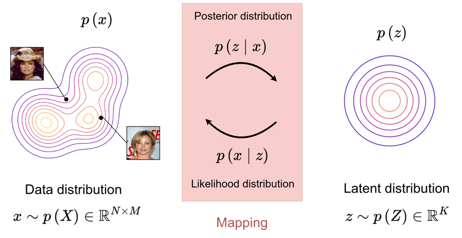
Variational inference can be used in various applications, including the modeling of complex distributions \(p(x)\).
-
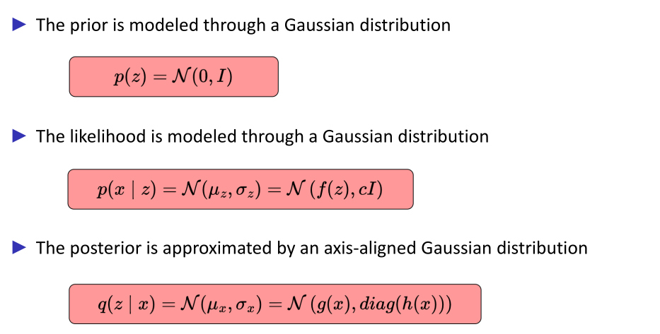
A latent variable model is introduced, where a prior \(p(z)\) and a likelihood \(p(x \mid z)\) define a joint distribution over the data.
-
The marginal likelihood \(p(x)\) is typically intractable, and variational inference introduces a tractable approximation \(q(z \mid x)\) of the posterior distribution \(p(z \mid x)\).
Modeling
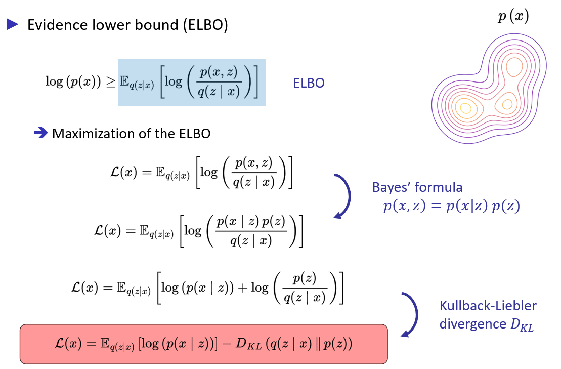
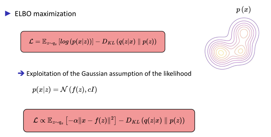
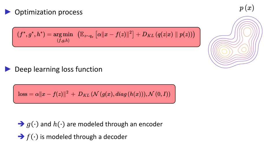
Optimization process for modeling a complex distribution
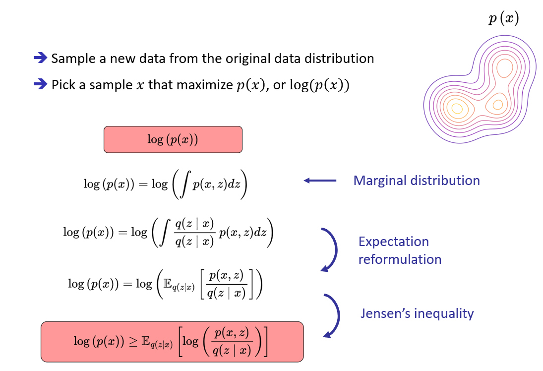
Maximization of the Evidence Lower BOund (ELBO)
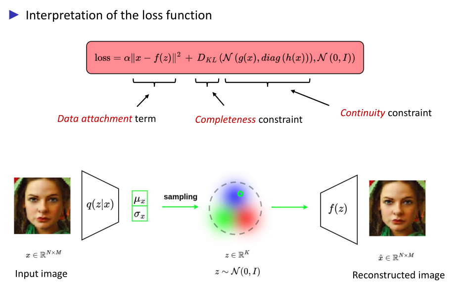
VAE application
Hypothesis
Amortized simulation-based inference
Definition
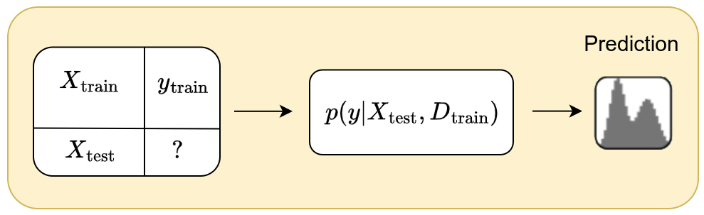
The idea behind the amortized simulation-based inference is to model the ouput \(y\) from a new input \(x\) based on a supervised dataset \(D=(X_{\text{train}},y_{\text{train}})\) of arbitrary size \(n\).
The goal is therefore to model the posterior predictive distribution \(p(y \mid x, D)\). Since we explicitly use a support dataset \(D\) to predict \(y\) from \(x\), this model falls under in-context learning.
Moreover, amortized simulation-based inference is based on the hypothesis that there exists a relationship between the inputs \(X\) and the output labels \(y\). This relationship can be modeled through a prior that can be used to generate synthetic datasets.
Modeling
Modeling relationships in the data
The prior defines a space of hypotheses \(\Phi\) on the relationship of a set of inputs \(X\) to the output labels \(y\). Each hypothesis \(\phi \in \Phi\) can be seen as a mechanism that generates a data distribution from which we can draw samples forming a dataset.
A prior is not merely a distribution over parameters; it encodes assumptions about the underlying data-generating process, thereby introducing an inductive bias
Inductive bias is the set of structural assumptions that a model imposes on the space of plausible solutions before observing any data. In Bayesian inference, it is formally encoded by the prior, and it determines how the model generalizes from a finite number of observations
Prior sampling scheme
Based on the hypothesis \(\Phi\), one can implement an efficient prior sampling scheme of the form:
\[p(D) = \int_{\phi} p(D \mid \phi) \, p(\phi) \, d\phi\]The generative mechanism is first sampled as \(\phi \sim p(\phi)\) which encodes the relationships between \(X\) and \(y\). The synthetic dataset is then sampled as \(D\sim p(D \mid \phi)\). This process is finally repeated for a large set of \(\phi\) sampled from \(\Phi\).
Learning process
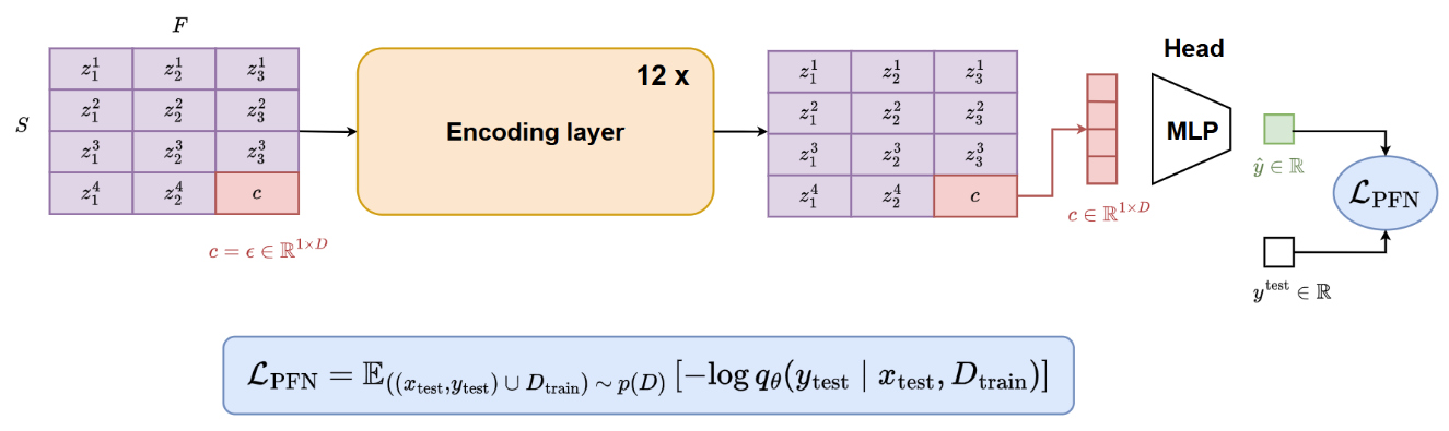
The posterior predictive distribution \(p(y \mid x, D)\) is approximated through a parametrized function \(q_{\theta}(y \mid x, D)\)
The model \(q_{\theta}(\cdot)\) is trained by minimizing the cross-entropy over samples drawn from the prior:
\[l_{\theta} = \mathbb{E}_{D \cup \{x,y\} \sim p(D)}\left[ - \log q_{\theta}(y \mid x,D) \right]\]where \(D \cup \{x,y\}\) denotes a synthetic dataset of size \(\lvert D \rvert +1\), obtained by augmenting \(D \sim p(D)\) with a pair \(\{x,y\}\).
The proposed objective \(l_{\theta}\) is equal to the expectation of the cross-entropy between the posterior predictive distribution \(p(y \mid x, D)\) and its approximation \(q_{\theta}(y \mid x, D)\) : \(l_{\theta} = \mathbb{E}_{x,D \sim p(D)}\left[ H\left(p(\cdot \mid x,D) , q_{\theta}(\cdot \mid x,D) \right) \right]\)
Proof. The above can be shown with the following derivation.
\(\begin{aligned}
l_{\theta} & = \mathbb{E}_{D \cup \{x,y\} \sim p(D)}\left[ - \log q_{\theta}(y \mid x,D) \right] \\
& = \mathbb{E}_{D,x,y} \left[ - \log q_{\theta}(y \mid x,D) \right] \\
& = -\int_{D,x,y}p(x,y,D) \, \log q_{\theta}(y \mid x,D) \\
& = -\int_{D,x,y} \color{orange}{p(x,D) \, p(y \mid x,D)} \, \log q_{\theta}(y \mid x,D) \\
& = -\int_{D,x}p(x,D) \, \int_{y} p(y \mid x,D) \, \log q_{\theta}(y \mid x,D) \\
& = \int_{D,x} p(x,D) \, \color{orange}{H \left( p(\cdot \mid x,D) , q_{\theta}(\cdot \mid x,D) \right)} \\
& = \mathbb{E}_{x,D\sim p(D)} \left[ H \left( p(\cdot \mid x,D) , q_{\theta}(\cdot \mid x,D) \right) \right]
\end{aligned}\)
Corollary. The loss \(l_{\theta}\) equals the expected KL-Divergence \(\mathbb{E}_{D,x}\left[ KL\left( p(\cdot \mid x,D) , q_{\theta}(\cdot \mid x,D) \right) \right]\) between \(p(\cdot \mid x,D)\) and \(q_{\theta}(\cdot \mid x,D)\) over prior data \(x, D\), up to an additive constant.
\[\begin{aligned} & \mathbb{E}_{x,D}\left[ KL \left( p(\cdot \mid x,D), q_{\theta}( \cdot \mid x,D) \right) \right] \\ &= - \mathbb{E}_{x,D}\left[ \int_y p(y \mid x,D) \, \log \frac{q_{\theta}(y \mid x,D)}{p(y \mid x,D)} \right] \\ &= - \mathbb{E}_{x,D}\left[ \int_y p(y \mid x,D) \, \log q_{\theta}(y \mid x,D) \right] + \mathbb{E}_{x,D}\left[ \int_y p(y \mid x,D) \, \log p(y \mid x,D) \right] \\ &= \mathbb{E}_{x,D}\left[ H \left( p(\cdot \mid x,D), q_{\theta}(\cdot \mid x,D) \right) \right] - \mathbb{E}_{x,D}\left[ H \left( p(\cdot \mid x,D) \right) \right] \\ &= l_{\theta} + C \end{aligned}\]where \(C\) is a constant that does not depend on \(\theta\).
tabPFN1 application
Prior modeling through Structural Causal Models (SCMs)
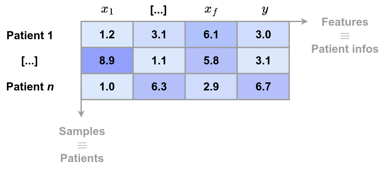
Tabular data can be seen as the result of several simple mechanisms interacting with each other.
- a table row corresponds to a real-world entity (patient, customer, transaction, etc.)
- each column corresponds to a measurement, decision, or attribute produced by a real process
- the label represents a consequence (diagnosis, defect, class, etc.)
Tabular data result from chains of decisions, mechanisms, and constraints. Even if the exact causal structure is unknown, tabular data are almost always causal in essence.
Causality refers to the fact that variables are linked through cause–effect relationships, even if their exact structure is unknown.
Structural Causal Models (SCMs) are thus used as the prior to model the implicit structure of tabular data. They impose a “reasonable” structure without being rigid.
They model:
- nonlinear dependencies
- interactions
- noise
- different graphs (i.e. relationships) across datasets
They allow:
- local, composed, and parsimonious structures
- plausible dependencies between columns
- preference for simple relationships
Synthetic dataset generation
To generate a synthetic dataset, TabPFN essentially follows the following pipeline:
- Sample a causal structure (DAG)
- Sample the causal mechanisms
- Sample noise terms
- Generate the features
- Generate the label
- Apply realistic transformations
- Sample a small dataset (few-shot regime)
Each dataset corresponds to a task for which TabPFN learns to perform Bayesian inference.
1- Sample a causal structure (DAG)
- Number of variables: randomly sampled within a range (e.g., 5 to 100)
- Graph structure
- sparsity is encouraged
- a small number of parents per node
- a random topological ordering
The intuition behind this sampling scheme is that real-world tabular variables rarely exhibit global dependencies across all columns
2- Sample the causal mechanisms
The following relation is defined for each variable \(X_i\) with parents \(Pa(X_i)\): \(X_i = f_i \left( Pa(X_i) \right) + \epsilon_i\)
\(f_i\) is randomly chosen from a mixture of function families:
- linear functions
- simple nonlinear functions
- small neural networks
- sometimes tree- or threshold-based functions
But with:
- low depth
- low complexity
- simple activations
3- Sample noise terms
Each variable has its own noise term \(\epsilon_i \sim N(0,\sigma_i^2)\). The variance \(\sigma_i\) is sampled randomly.
4- Generate the features (propagation through the DAG)
Once we have:
- the graph
- the structural functions
- the noise terms,
features are generated according to the causal ordering:
- variables without parents \(\rightarrow\) sampled directly
- intermediate variables \(\rightarrow\) computed via \(𝑓_i\)
- deeper variables \(\rightarrow\) accumulate dependencies and noise
A set of features are then randomly selected from the graph
5- Generate the label \(y\)
The label is treated as a final causal variable.
A value of \(y\) is first randomly selected from the graph and then updated according to the following equation:
\[y = g \left( Pa(y) \right) + \epsilon_y\]where:
- \(g\) is sampled as a simple function
- \(y\) sometimes depends on a few variables
- \(y\) sometimes depends indirectly on many variables through the DAG
For classification:
- \(g\) produces a latent score
- passed through a sigmoid or softmax
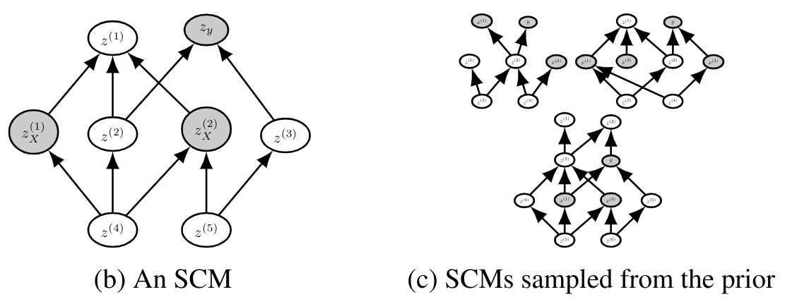
- then the class is sampled
The figure below shows an example of SCMs sampled from the prior. The grey nodes correspond to the sampled inputs \(X\) and output \(y\).
6- Apply realistic transformations
Before feeding the dataset to the model, TabPFN applies:
- random normalization
- column permutation
- different scalings per feature
- monotonic transformations
- introduction of class imbalance
These steps prevent the model from “cheating” by recognizing the generator.
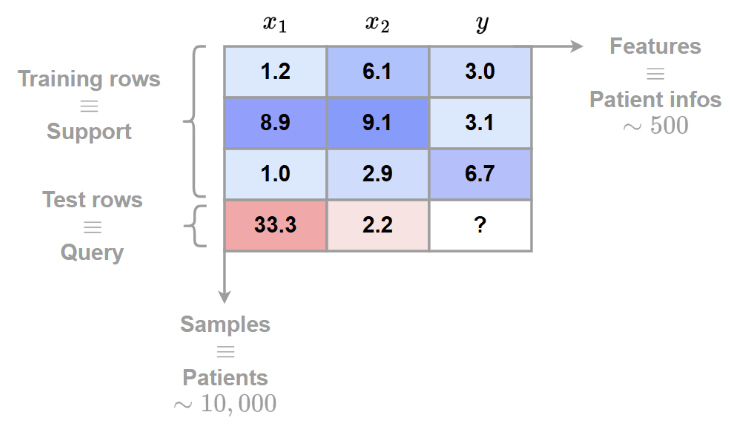
7- Sample a small dataset (few-shot regime)
Finally:
- a small number of samples \(𝑛\) is drawn (often \(<1000\))
- train/test split is created
- everything is provided in-context to the transformer
Data preprocessing
Both the synthetic and the real datasets are represented as follows:
The categorical data are encoded as integers
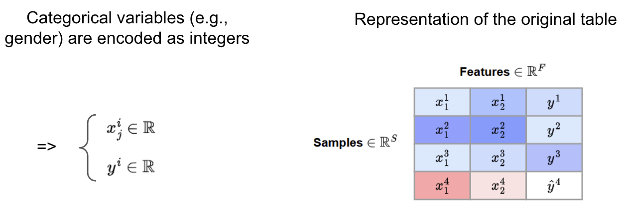
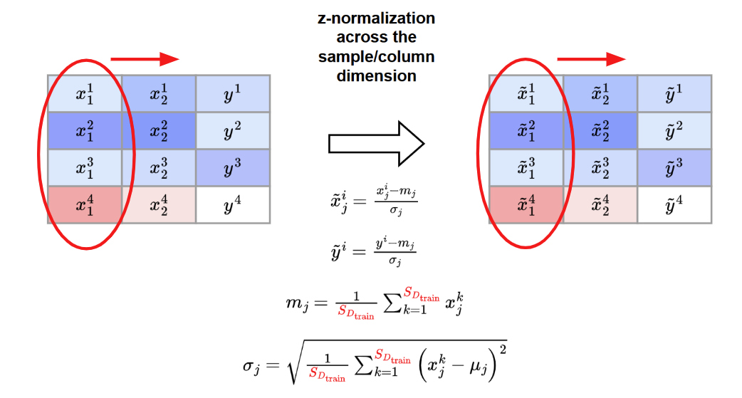
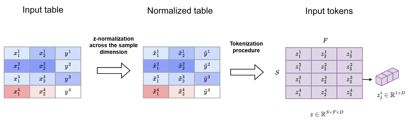
A z-normalization across feature/column dimension is applied
Tokenization procedure
After data preprocessing, each tabular feature is embedded as a token using a shared linear projection
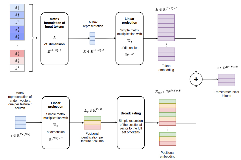
This yields the following representation at the input of the transformer
Transformer architecture
The following transformer architecture is proposed. It consists of 12 layers that sequentially apply attention over features and attention over samples. It should be noted that attention over samples is applied between all support samples and one query sample at a time. Query samples do not interact with one another.
Training procedure
During training, each batch is populated with a dataset sampled from the SCM distribution described above. The following scheme is then applied
Implementation
- TabPFN was trained for approximately 2,000,000 steps with a batch size of 64 datasets
- That means TabPFN is trained on around 130,000,000 synthetically generated datasets !
- One training run requires around 2 weeks on one node with eight Nvidia RTX 2080 Ti GPUs
- The number of training samples was sampled for each dataset uniformly up to 2,048 and use a fixed validation set size of 128
- The number of features was sampled using a beta distribution that was linearly scaled to the range 1–160
- To avoid peaks in memory usage, the total size of each table was restricted to be below 75,000 cells by decreasing the number of samples for tables with a large numbers of features
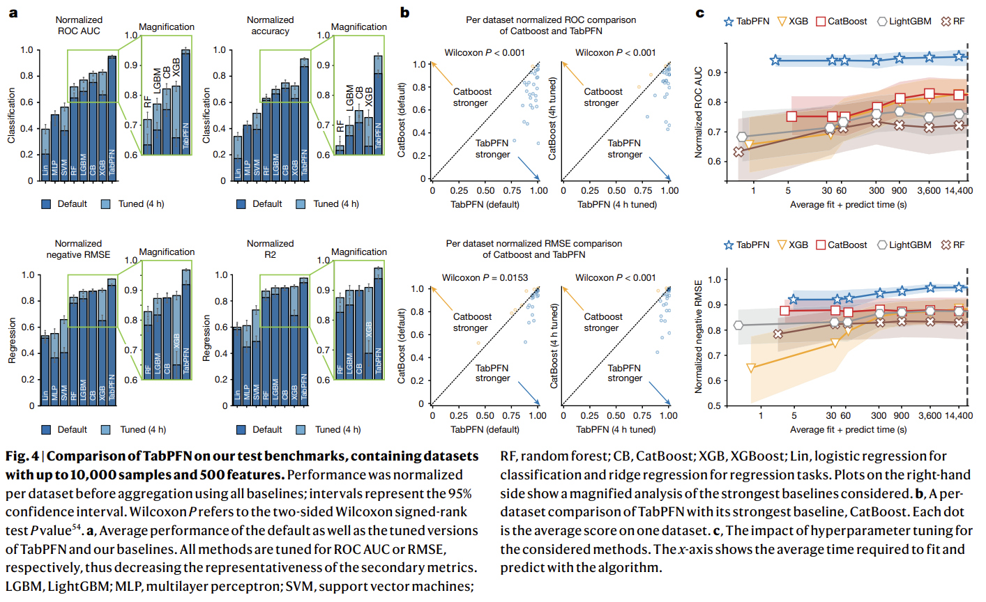
Experiments
- TabPFN was compared against state-of-the-art baselines, including tree-based methods (random forest, XGBoost (XGB), CatBoost, LightGBM), linear models, support vector machines (SVMs) and MLPs
- TabPFN was evaluated on two dataset collections:
AutoML BenchmarkandOpenML-CTR23. These benchmarks comprise diverse real-world tabular datasets, curated for complexity, relevance and domain diversity - From these benchmarks, the authors used 29 classification datasets and 28 regression datasets that have up to 10,000 samples, 500 features and 10 classes
- Evaluation metrics include ROC AUC and accuracy for classification, and R2 and negative RMSE for regression
- Scores were normalized per dataset, with 1.0 representing the best and 0.0 the worst performance with respect to all baselines
- Hyperparameters were tuned using random search with five-fold cross-validation, with time budgets ranging from 30 s to 4 h
- All methods were evaluated in inference using eight CPU cores, with TabPFN additionally using one GPU (RTX 2080 Ti)
Results
1- Comparison with state-of-the-art baselines
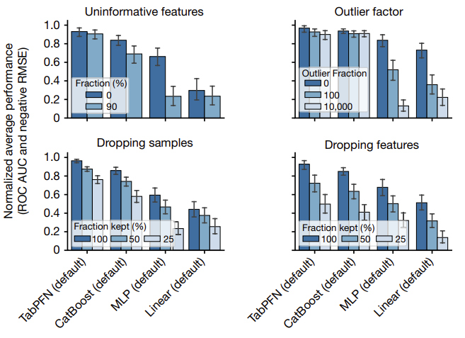
2- Evaluating diverse data attributes
The figure below provides an analysis of the performance of TabPFN across various dataset types:
- add uninformative features (randomly shuffled features from the original dataset)
- add outliers (2% probability of multiplying a cell with a random number between 0 and the outlier factor)
- remove/drop samples
- remove/drop features
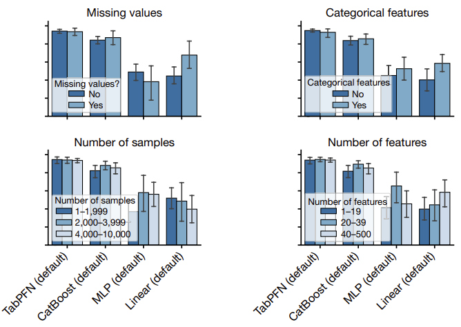
The figure below provides an analysis of the performance of TabPFN on different subgroups:
- presence of missing values
- presence of categorical features
- number of samples
- number of features
References
-
Hollmann N. et al. Accurate predictions on small data with a tabular foundation model., Nature 2025 ↩