STAMP: Subtype-Aware Spatio-Temporal Atlases for Personalized Prediction of Longitudinal Alzheimer's Disease Progression
Highlights
- The goal: predict how a patient’s brain anatomy will change. Alzheimer’s disease can affect brain regions differently across patients. STAMP learns from repeated 3D brain MRI scans to discover different patterns of progression and use them to forecast future anatomy.
- Learn several possible paths of progression. The model learns how changes in each brain region evolve over disease time, with a different set of curves for each subtype.
- Locate each patient on those paths. Baseline regional brain volumes estimate where the patient is on a shared disease timeline. Regional volumes and clinical scores also determine how strongly each subtype contributes to the prediction. This separates two questions: how far has the disease progressed? and which pattern of change best fits this patient?
- Turn the progression curves into a future MRI. For a requested follow-up interval, STAMP combines the subtype curves to compute a regional change signal. It maps that signal onto the patient’s brain segmentation and predicts a smooth deformation of the baseline MRI, producing a personalized forecast of future anatomy.
- Code repository announced by the authors and MICCAI paper page.
Introduction
Alzheimer’s disease does not progress identically across patients. A useful progression model should describe both when a patient is along a disease trajectory and which pattern of progression best explains their anatomy.
Existing approaches address different parts of this problem:
- Biomarker-based subtyping, such as SuStaIn1, estimates subtypes and disease stages using scalar measurements. This supports patient stratification but does not directly learn fine-grained anatomical changes from full images.
- Image-based longitudinal models, such as spatio-temporal atlases and generative MRI forecasting methods, capture spatial changes. However, flexible individual variation does not necessarily produce explicit, interpretable progression subtypes.
STAMP combines these ideas: subtype-specific regional dynamics condition a deformation model that forecasts a patient’s future brain anatomy. Its atlas backbone builds on SMART2, extending continuous-time image progression modeling with a learned gate between multiple trajectories.
Methods
Overview
The model is trained on longitudinal T1-weighted MRI series. For a new subject, it uses baseline anatomy, its segmentation, baseline clinical information, and a requested follow-up interval to predict anatomical evolution.
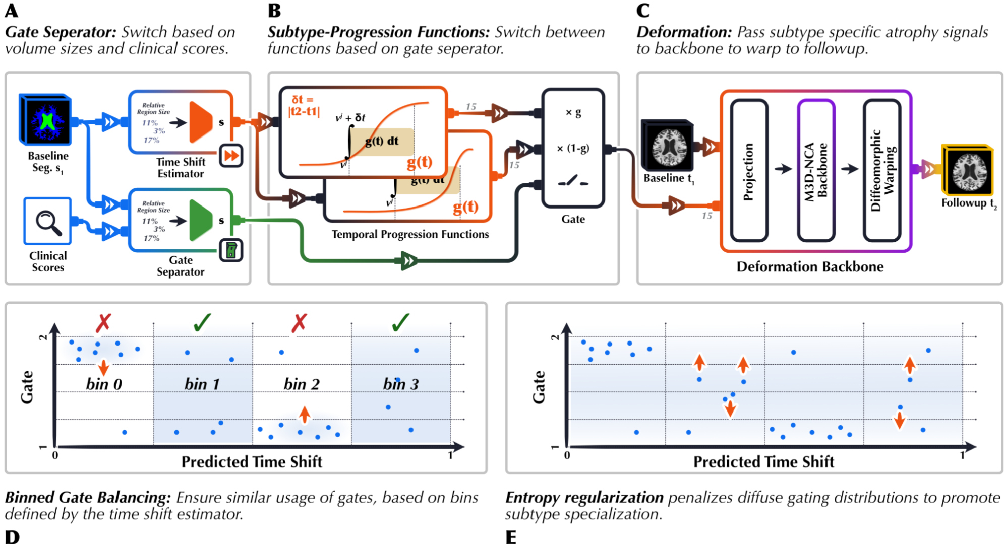
There are three levels of modeling:
- Temporal alignment: locate the subject on a shared disease time axis.
- Regional progression: integrate the dynamics of each subtype over the requested interval and combine them using subject-specific weights.
- Voxel-level deformation: project the regional signal into image space and predict a deformation of the baseline MRI.
All components are optimized jointly. Although the method operates on 3D images, its temporal alignment and subtype gate also depend on regional summaries and clinical inputs.
Continuous-time regional trajectories
For each subtype \(s \in \{1,\ldots,C\}\), STAMP learns a progression function
\[g^s(t) \in \mathbb{R}_{\geq 0}^{K},\]where \(K\) is the number of brain regions and \(g_k^s(t)\) is the instantaneous regional progression signal at disease time \(t\). The functions are parameterized using neural ordinary differential equations (neural ODEs)3, allowing nonlinear temporal dynamics.
Time reparameterization: patients enter the study at different disease stages: two baseline scans need not represent the same point in progression, even for patients of the same age. STAMP therefore estimates a patient-specific starting position \(v^j\) on a shared disease timeline from baseline relative regional volumes.
The same subject position is used when evaluating the different subtype trajectories. For a forecasting interval \(\delta t\), the integrated progression signal for subject \(j\) and subtype \(s\) is
\[I^{j,s}(\delta t;v^j) = \int_{v^j}^{v^j+\delta t} g^s(t)\,dt.\]Thus, disease time is distinct from chronological age: subjects with different ages can occupy similar positions on the learned progression axis. Personalization combines this temporal position with subtype membership and baseline anatomy; the paper describes a time shift rather than a separate subject-specific progression-speed parameter.
Subtype gating
A gating network is a neural network that learns how much weight to give each of several possible model outputs for a particular input. In STAMP, those alternatives are the subtype-specific progression signals. The gate receives a patient’s baseline relative regional volumes and clinical information, then returns one weight per subtype: a larger weight means that subtype contributes more to the patient’s forecast.
For patient \(j\), these weights form a probability-like vector: they are non-negative and sum to one,
\[\theta^j \in \Delta^{C-1}, \qquad \theta_s^j \geq 0, \qquad \sum_{s=1}^{C}\theta_s^j=1.\]The regional signal passed to the deformation model is the weighted average (or convex combination) of the subtype-specific signals,
\[I^j = \sum_{s=1}^{C}\theta_s^j I^{j,s}.\]The reported experiments learn two subtypes. For example, weights of 0.8 and 0.2 would produce a regional signal containing 80% of the first subtype’s signal and 20% of the second’s. The gate is trained jointly with the progression curves and deformation model, so it learns weights that help predict observed follow-up anatomy, without requiring predefined subtype labels. Although training encourages confident assignments, the mathematical formulation uses a weighted mixture rather than requiring a hard subtype selection.
From regional signals to MRI deformations
The baseline segmentation projects each regional signal onto the corresponding voxels, creating a dense growth map. This conditions a deformation backbone based on M3D-NCA, a 3D neural cellular automaton4. Local, recurrent voxel updates predict a stationary velocity field, which is integrated to obtain a diffeomorphic displacement used to warp the baseline image.
In a neural cellular automaton (NCA), each cell repeatedly updates its state using a shared learned rule and information from its neighbors. For an interactive introduction to this principle, see Distill’s Growing Neural Cellular Automata.
The growth signal is a non-negative, region-level conditioning variable for the learned deformation model, rather than a directly reported signed volume-change measurement. The deformation model uses this signal, together with baseline anatomy, to predict a voxel-level deformation field; therefore the sign and anatomical interpretation of the resulting local volume change are not specified directly by the value of the growth signal.
Preventing subtype collapse
Jointly learning trajectories and assignments can produce degenerate solutions: all subjects may use one subtype, assignments may remain diffuse, or the gate may merely divide subjects by disease stage.
Entropy regularization encourages confident assignments. For a minibatch of \(M\) subjects,
\[\mathcal{L}_{\mathrm{ent}} = \frac{1}{M}\sum_{j=1}^{M}H(\theta^j), \qquad H(\theta^j)=-\sum_{s=1}^{C}\theta_s^j\log\theta_s^j.\]Minimizing this loss sharpens the gate, but does not by itself prevent every subject from choosing the same subtype.
Time-binned balancing constrains subtype usage within bins of the estimated disease axis. If \(S_b\) contains subjects in bin \(b\), average subtype usage is
\[u_{b,s}=\frac{1}{|S_b|}\sum_{j\in S_b}\theta_s^j.\]A smooth barrier penalizes values outside \([\alpha,1-\alpha]\):
\[\mathcal{L}_{\mathrm{bin}} =\frac{1}{B}\sum_{b=1}^{B}\sum_{s=1}^{C}\phi(u_{b,s}),\]where \(B\) is the number of time bins. An exponential moving average reduces noise in the estimated usage. Requiring multiple subtypes at each stage discourages a split that simply assigns early and late disease to different clusters.
Curriculum scheduling emphasizes balancing early, when trajectories are not yet reliable, then reduces its weight and increases entropy regularization to consolidate specialization. The training objective combines the forecasting loss with these two regularizers. The paper does not specify the exact forecasting-loss formula or numerical schedule.
Experiments
Data and setup
- Cohort: ADNI-1/GO/2, with 446 subjects and 1,041 scans; at least two time points per subject and a mean follow-up of 2.95 years.
- Selection: available cognitive assessments (ADAS11, FAQ, MMSE, CDRSB, MOCA) and confirmed amyloid pathology, using \(A\beta < 192\ \mathrm{pg/mL}\).
- Preprocessing with turboprep5: MRI scans are skull-stripped and affinely aligned, then resampled to \(128 \times 160 \times 128\) voxels. Brain tissue segmentation is obtained with SynthSeg 2.0.
- Split: 80% training, 5% validation, and 15% testing, separated at the patient level.
- Training: PyTorch and Adam.
- Comparisons: CounterSynth, BrLP, and Conditional VoxelMorph, reproduced from official implementations with matched preprocessing, resolution, and splits.
Results
Anatomical forecasting
Table 1 compares regional volume forecasting across all 18 regions. The mean absolute error (MAE) is expressed as a percentage of total brain volume and reported as mean ± standard deviation. Lower values are better; bold entries mark the best results, and asterisks indicate significant pairwise differences (\(p<0.05\)).
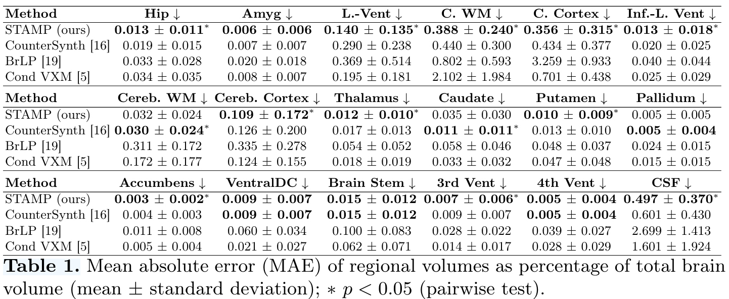
The authors report the lowest MAE in 16 of 18 regions, with some ties at the displayed precision. CounterSynth performs better in cerebellar white matter and the caudate. STAMP is significantly better than CounterSynth in 11 regions, using two-tailed paired t-tests with \(p<0.05\).
Geometric agreement, averaged across regions, is:
| Method | Dice (higher is better) | Hausdorff95 (lower is better) |
|---|---|---|
| STAMP | 0.907 | 1.010 |
| CounterSynth | 0.907 | 1.018 |
| Conditional VoxelMorph | 0.856 | 1.065 |
| BrLP | 0.665 | 2.207 |
The main advantage over CounterSynth is therefore in regional volumetric forecasting; their average geometric scores are very similar. These comparisons concern the reproduced models on this cohort and split.
Learned progression regimes
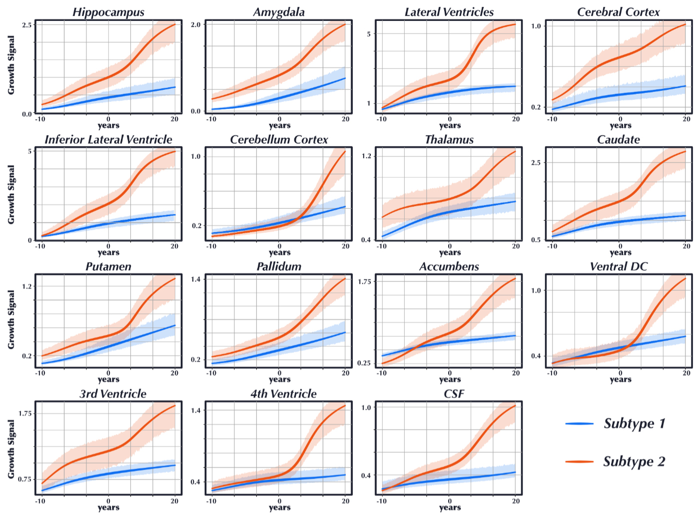
The learned functions show different progression dynamics across regions. The paper reports associations between the subtype gate and clinical or biomarker variables, including ADAS13 (\(p<10^{-13}\)), amyloid-β (\(p<10^{-6}\)), TAU (\(p<10^{-6}\)), and APOE4 carrier frequency (\(p<10^{-2}\)).
- 95% of cognitively normal subjects are assigned to Subtype 1.
- 100% of dementia cases are assigned to Subtype 2.
- Subjects with mild cognitive impairment span both trajectories.
The estimated time shift correlates moderately with ADAS13 (Spearman \(\rho=0.43\), \(p<10^{-3}\)). Subtype assignment is not significantly correlated with time shift (\(p>0.05\)), and both subtypes cover the estimated disease axis. This supports a distinction between stage and progression regime, although a nonsignificant correlation does not establish independence.
The authors interpret these groups as data-driven progression regimes, rather than definitive biological disease subtypes.
Personalization and ablations
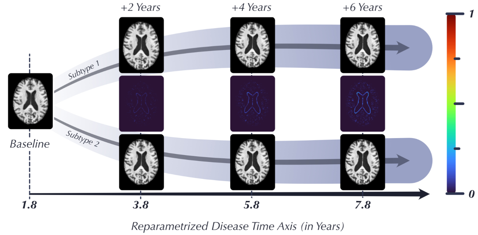
Table 2 compares full STAMP with inverted gate assignments and variants without subtypes, curriculum scheduling, time-binned balancing, or entropy regularization. It reports selected regional errors and the average over all 18 regions (AVG), in the same regional-volume MAE units as Table 1.
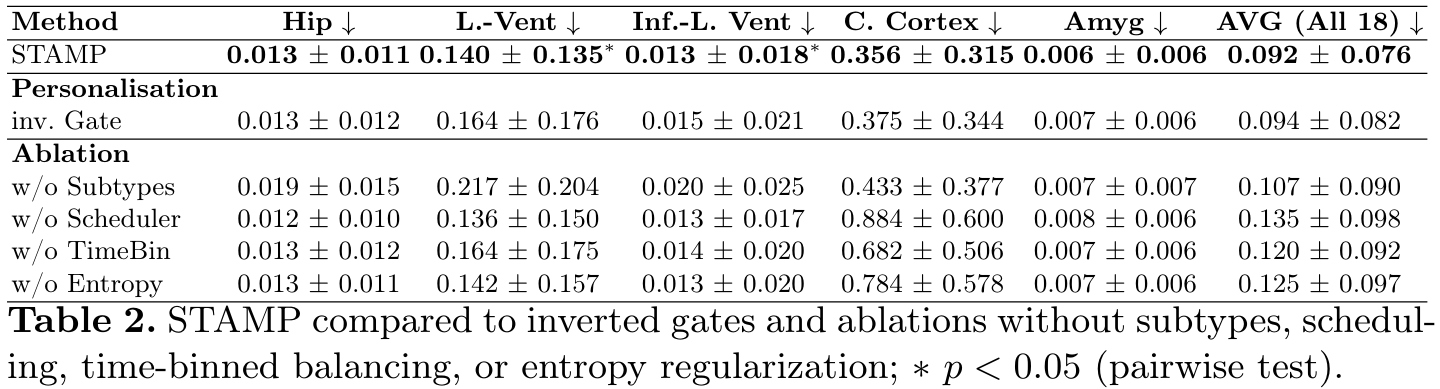
Removing subtypes increases average error from 0.092 to 0.107. Removing any of the stabilization components also degrades the overall result, with the largest average degradation occurring without curriculum scheduling.
Inverting the gate gives a smaller average degradation (0.092 to 0.094). Significant differences are marked for the lateral and inferior lateral ventricles in this comparison. This supports the usefulness of personalized routing, while showing that its effect varies by region.
Conclusions
- STAMP connects explicit progression subtyping to continuous-time, deformation-based MRI forecasting within one jointly trained model.
- Regional dynamics and the shared disease axis provide an interpretable intermediate representation between patient-level gating and voxel-level anatomical change.
- The ADNI results support improved regional volume prediction, and the ablations show that learning useful subtypes requires careful regularization and scheduling.
Remarks
- External validation: evaluation is restricted to an amyloid-positive ADNI cohort. Generalization to independent cohorts, other populations, and different acquisition settings remains to be established.
- Meaning and number of subtypes: the experiments report two progression regimes. The paper does not provide a study selecting the number of subtypes or demonstrate that these groups are stable biological categories. Their strong diagnostic associations also warrant further study.
- Statistical interpretation: the reported regional tests use \(p<0.05\); the paper does not describe correction for multiple comparisons across regions.
- Reproducibility: the main paper does not specify the numerical solver used for ODE integration. It also does not provide numerical details for the bin bounds, scheduling weights, or several training hyperparameters. The announced implementation is relevant for reproducing these choices.
References
-
Young, A. L., et al. Uncovering the heterogeneity and temporal complexity of neurodegenerative diseases with Subtype and Stage Inference. Nature Communications 9, 4273 (2018). ↩
-
Kalkhof, J., Lorenzi, M. SMART: A Flexible, Interpretable, and Scalable Spatio-temporal Brain Atlas from High-Resolution Imaging Data. February 2026. ↩
-
Chen, R. T., Rubanova, Y., Bettencourt, J., Duvenaud, D. K. Neural Ordinary Differential Equations. Advances in Neural Information Processing Systems 31 (2018). ↩
-
Kalkhof, J., Mukhopadhyay, A. M3D-NCA: Robust 3D Segmentation with Built-in Quality Control. MICCAI, pp. 169-178 (2023). ↩
-
Puglisi, L. turboprep. 2023. Accessed October 8, 2025, as cited in the STAMP paper. ↩