Highlights

RefTr is the third iteration of a tracking approach by the same group (after Trexplorer¹ and Trexplorer Super²) to extract the centerline tree of vessels or airways from 3D images, directly as a graph.
Like its predecessors, it relies on the same mechanisms as DETR (learned queries, Transformer decoder, Hungarian matching), applied to tracking.
Instead of tracking the tree point by point, it predicts and iteratively refines whole trajectories, which increases the detection rate and lets errors be corrected while a branch is being predicted. Represented as confluent trajectories, the tree is valid by construction.
It outperforms its predecessor Trexplorer Super on most benchmarks, and is twice cheaper to train, in both training time and GPU memory.
Code is available on the official GitHub repo.

Introduction

Extracting tubular trees such as vessels or airways is important for many clinical applications, such as surgical planning and navigation, or blood flow simulation. Most of the time, these applications need the full tree, and a segmentation alone is not enough : it shows where the tubes are, but not how they branch and connect. We need a model of the complete tree, represented as a centerline graph that is a valid tree and misses as few branches as possible.

To obtain such a structure, several approaches have been proposed, which the authors group into four families:

Segmentation-based methods (e.g. clDice³, DeepVesselNet⁴) segment the structure voxel by voxel, then skeletonize it. They need costly voxel-level labels, post-processing, and do not predict the graph end to end.
Graph-based methods (Relationformer⁵, Vesselformer⁶) predict nodes and edges directly, but nothing guarantees a valid tree, and they scale poorly to large trees.
Multiple-hypothesis tracking⁷ keeps several candidate trees during reconstruction, but finally prunes all but one, discarding potentially useful structures.
Tracking-based methods, mainly Trexplorer¹ and Trexplorer Super² from the same group, follow the tree from its root, one node at a time. Each new node is classified as intermediate, bifurcation or end. These classifications are hard and imbalanced, which lowers recall, and an early mistake cannot be corrected.

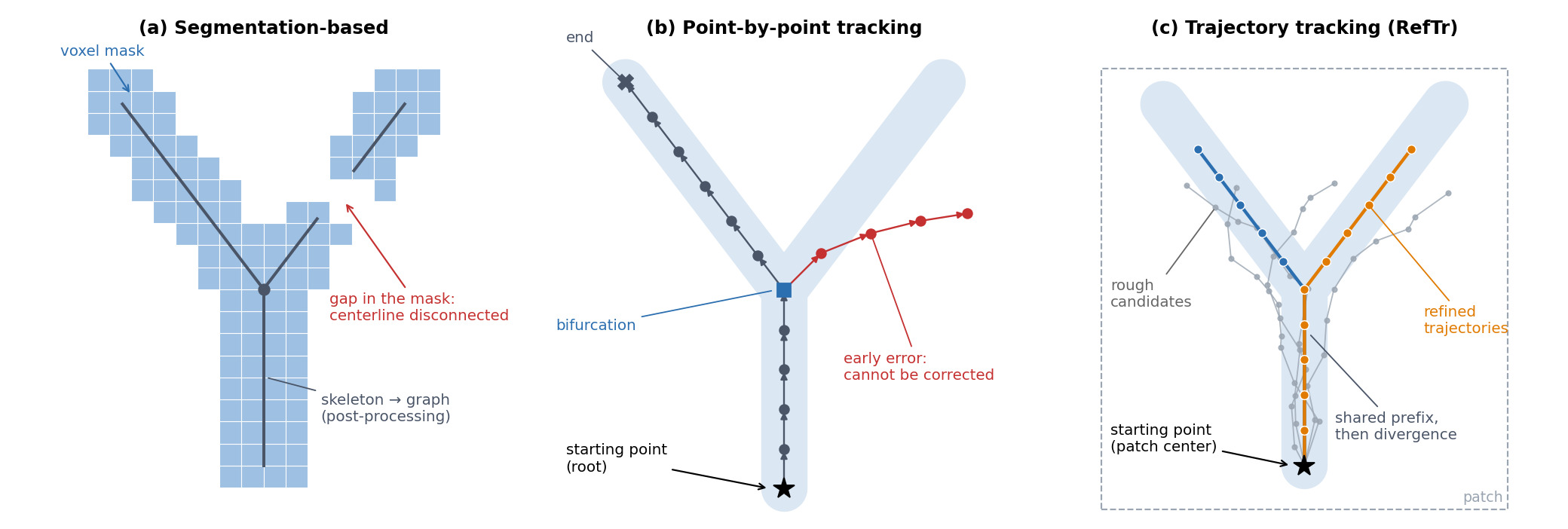
Figure 1. Three ways to extract a centerline tree. (a) Segmentation-based methods label voxels, then extract the centerline. (b) Point-by-point tracking adds one classified node at a time. (c) RefTr predicts whole trajectories from the patch center and refines them.

RefTr addresses these limitations and lists three contributions: (1) RefTr itself, (2) TNMS, an efficient algorithm to remove duplicate branches while preserving the tree topology, and (3) radius-aware evaluation metrics.

In my opinion, the main contribution is to shift tracking from a point-by-point to a trajectory-level approach: whole branch segments are predicted and refined at once, and their confluent representation guarantees a valid tree.

Inference

Input: CT volume + root of the tree (taken from the ground truth)
Start a patch at the root
While there are patches to explore:
    For each patch:
        1. Predict several candidate trajectories from the patch center
        2. Refine them iteratively
        3. Merge duplicate candidates into branches and add them to the tree (bifurcations, ends)        
        4. For each branch that continues, open a new patch at its end
Remove duplicate branches across patches (TNMS)
Output: centerline tree

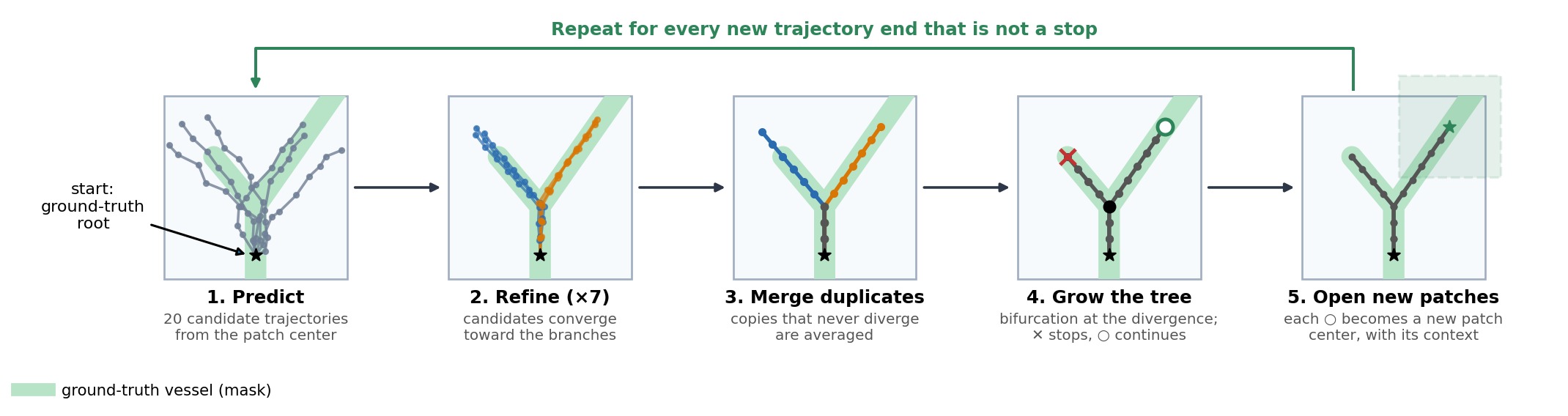
Figure 2. Overview of the inference algorithm.

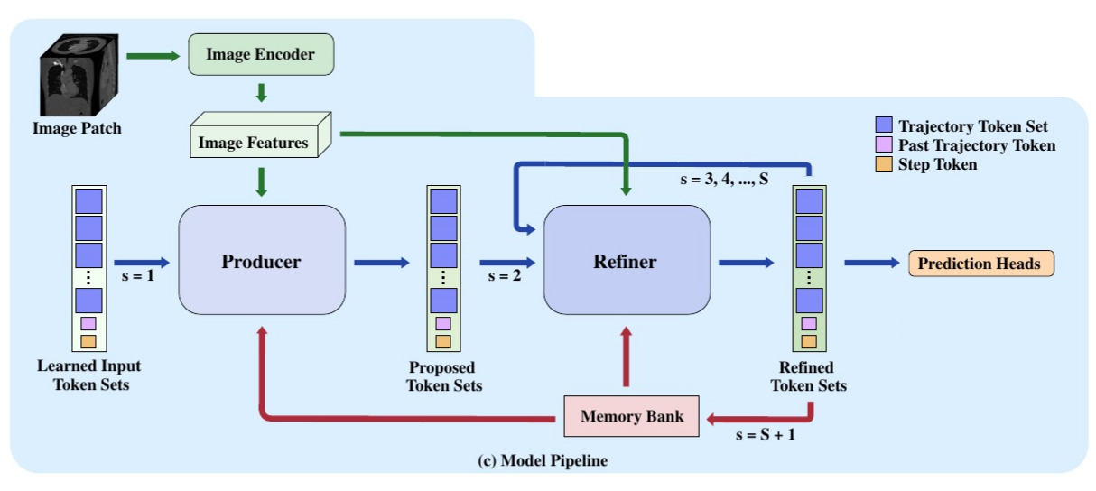
Figure 3. Overview of the model pipeline (figure from the paper, Fig. 1c).

Producer

Features are extracted from a patch centered on a centerline voxel. An image encoder (a modified SwinUNETR, the same as in Trexplorer Super) extracts features, which are fed to the Producer, a single Transformer decoder block, together with 20 token sets, each describing a trajectory. Using the image features, the Producer maps the 20 trajectories to potential vessel branches starting from the patch center and outputs the 20 modified token sets.

Trajectory representation

Each trajectory is represented by a trajectory token set. It contains:

10 node tokens, each encoding the position and radius of a node
1 end token, encoding the node number at which the branch ends.
1 divergence token, encoding the route of the trajectory so it can be compared with other trajectories and predicts the node where two trajectories diverge.

The trajectory tokens are not computed from an input. Like DETR’s object queries (see our DETR post), they are learned during training as a generic “identity card” of what a trajectory is, the same for every patch; the Producer and the Refiner then update them into trajectories adapted to the image content of the patch.

Context tokens

In addition to the 20 token sets, the Producer takes as input:

1 past trajectory token, which encodes up to the last ten positions and radii of the centerline leading to the patch center, to tell the model where it comes from (especially useful when the memory bank is still empty).
1 step token: encodes the refinement step number so that the shared Refiner can adapt the size of its updates.

Both are learned embeddings: in the code, a small MLP maps the concatenated past positions and radii to the past trajectory token, and a single linear layer maps the step number, normalized between 0 and 1, to the step token.

Refiner

The Refiner takes the Producer’s rough proposals and updates the trajectory tokens over \(S-1 = 7\) steps, cross-attending to the same image features at each step (the encoder runs only once) to bring every trajectory closer to its branch. Because whole trajectories can be corrected step by step, early mistakes are no longer final as in point-by-point tracking, at least within a patch: a branch committed in a previous patch is not revisited. Reusing the same block at every step keeps the decoder small. The Producer and Refiner blocks share the same design, detailed in the Training section.

Memory Bank

The memory bank stores the refined token sets of the ancestor trajectories from up to five previous patches.

It gives the model a memory of what it already predicted upstream, which helps keep the right direction in large vessels where a single patch shows only part of the tube, and reduces duplicate branches across patches.

It complements the past trajectory token. The past trajectory token is a short geometric summary (the last positions and radii leading to the patch center), with no image content, and mainly gives the direction to follow. The memory bank keeps the model’s own learned representation of the previous branches, which carries image information from earlier patches over a longer range. The ablation confirms their different roles: without the past trajectory token, recall collapses (67.72 % to 37.07 % on ATM’22), while without the memory bank, precision drops (74.16 % to 61.27 %).

Prediction heads

There are four prediction heads:

Head	Reads	Outputs	Used for
Position head	Each node token	3D position of the node	Placing the nodes in the volume
Radius head	Each node token	Local radius	The radius of each node in the tree
End head	The end token	End position along the trajectory	Deciding where a branch stops or whether it continues
Divergence head	Divergence token of trajectory \(i\) and \(j\)	Divergence index \(d_{ij}\)	Grouping duplicates and placing bifurcations

Divergence index

The tree is described as a set of \(n\) trajectories \(\mathcal{T} = \{T_i\}_{i=1}^n\), each being a sequence of nodes rooted at the patch center.

Two trajectories \(T_i\) and \(T_j\) share an identical prefix and separate only at a divergence index \(d_{ij}\), i.e. \(v_{i,k} = v_{j,k}\) for \(k \leq d_{ij}\).

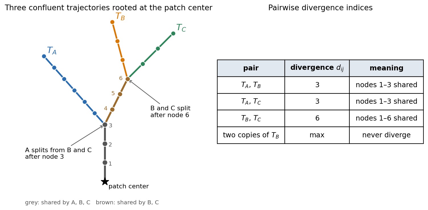
Figure 4. Three confluent trajectories and their pairwise divergence indices. Two copies of the same branch never diverge.

Merging trajectories and building the tree

After the last refinement step, the 20 trajectories are merged into a few branches in four steps.

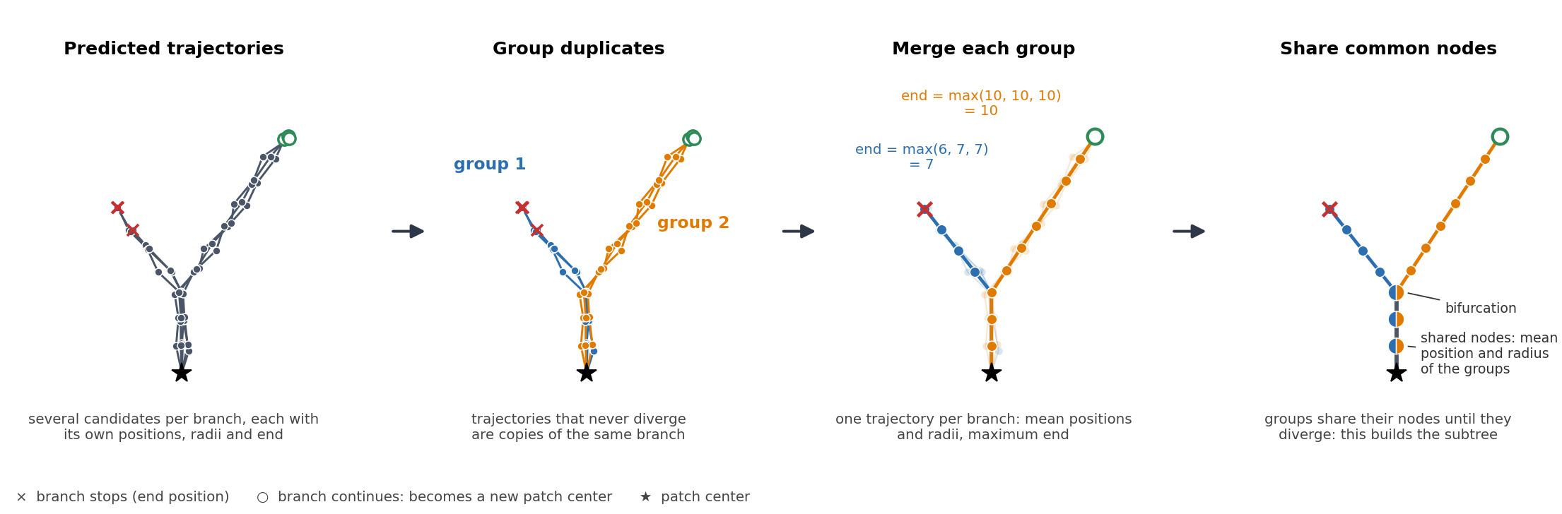
Figure 5. The trajectory merging algorithm

Step 1: make the divergences symmetric. For each pair, the two predictions \(d_{ij}\) and \(d_{ji}\) are averaged and rounded.
Step 2: form groups of duplicates. Two trajectories whose divergence is at the maximum never diverge: they are copies of the same branch and are put in the same group. Each group is one branch.
Step 3: merge each group into a single trajectory.

Quantity	How it’s merged
Position of node k	Mean of the members’ node k positions
Radius of node k	Mean of the members’ node k radii
End position	Maximum over the members
Divergence with another group	Mean of the divergences between their members

Step 4: build the subtree. Starting from the patch center, groups that have not yet diverged share a single node, whose position and radius are averaged over these groups. Where two groups diverge, a bifurcation is created. Each branch is then cut at its end position: if it stops before the last node, it terminates; otherwise its last node becomes the center of a new patch.

The tree topology is valid by construction, whatever the quality of the predictions. Valid does not mean correct, though: the output is always a tree, but not necessarily the right one.

Tree Non-Maximum Suppression (TNMS)

Patch-level grouping only sees the 20 trajectories of one patch. Since neighboring patches overlap a lot, the same vessel can still be traced twice: a trajectory may go back toward an already explored region, drift onto a neighboring vessel, or two copies may get a divergence slightly below the maximum and form a fake bifurcation. TNMS removes these residual duplicates on the full tree:

The tree is traversed in pre-order (depth first from the root).
When the traversal enters a new branch, the nodes of all previously visited branches are stored in a KD-tree.
A node is flagged if its nearest previously visited node is closer than a radius-adaptive threshold \(\tau = \max(\tau_{min}, \tau_{pos} \cdot r)\), with \(\tau_{pos} = 0.3\) and \(\tau_{min} = 2.0\).
A branch is a duplicate if at least \(\rho = 20\%\) of its nodes are flagged. This ratio is needed because every real child branch starts next to its bifurcation, so its first node is always flagged.
Flagged nodes of duplicate branches are merged with the nodes they matched into a single node (the one closest to the root is kept), and their neighbors are reconnected, so nothing attached further down is lost.
Merging can give a node two parents; only the edge from the parent closest to the root is kept.

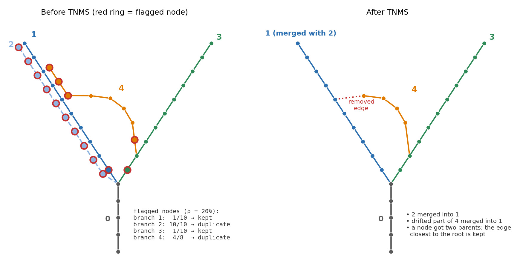
Figure 6. TNMS on a toy tree. Branch 1 and 3 are real (only their first node is flagged, 1/10). Branch 2 is a full duplicate of 1 (10/10 flagged) and is merged. Branch 4 drifts onto branch 1 (4/8 flagged): its drifted nodes are merged into branch 1, which gives a branch 1 node two parents; only the edge from the parent closest to the root is kept, so the edge coming from branch 4 is removed.

The authors report that, with KD-tree queries, TNMS runs in \(O(N \log N)\) and processes graphs with thousands of nodes in under a second on CPU.

Training

Training follows the same steps as inference (Figure 2), on a short chain of patches along the annotation, with two additions: each prediction is matched to a true branch, and a loss is computed against this branch at every step.

Repeat:
    Pick a path in an annotated tree, place 6 consecutive patches along it
    For each patch, in order:
        1. Predict candidate trajectories from the patch center (Producer)
        2. Match each candidate to a true branch (once, on the Producer's output)
        3. Refine the candidates (Refiner), measuring the error against the matched branch at every step
        4. Update the weights
        5. Pass the context on to the next patch

Input: 6 consecutive patches

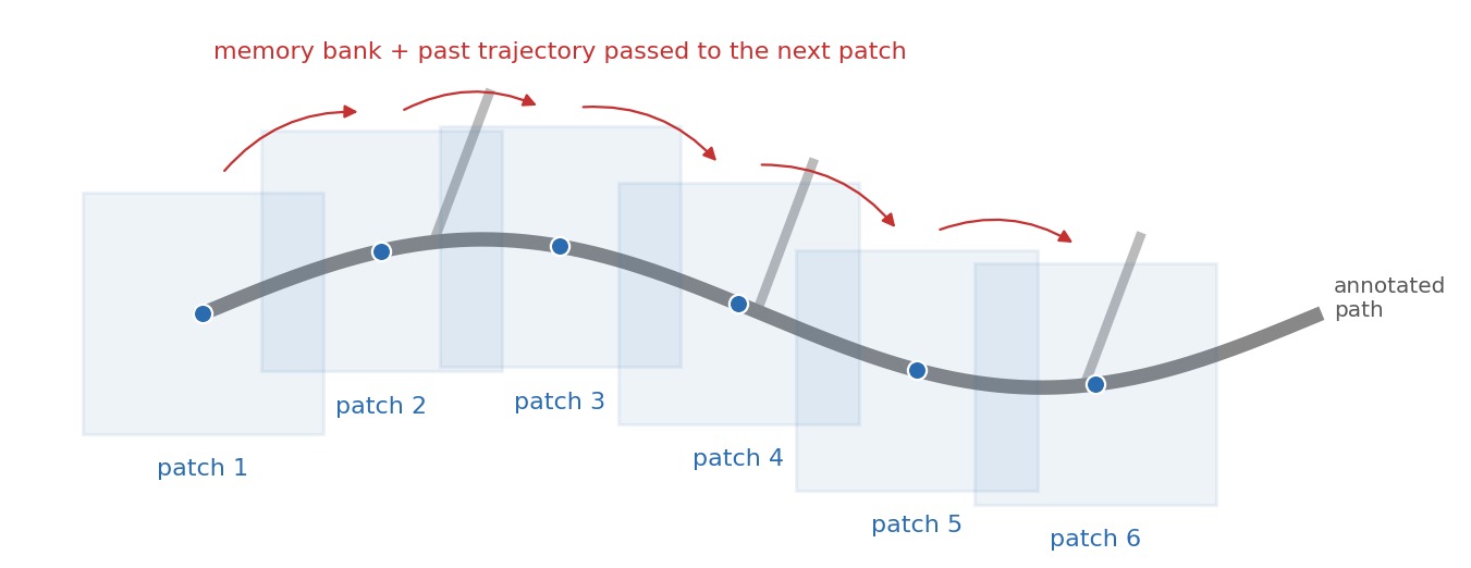
Figure 7. A training sample: 6 consecutive patches along an annotated path, processed in order.

At inference, a patch is never processed alone: it receives a past trajectory and a memory bank from the patches explored before it. To learn to use this context, the model must see it during training. As in Trexplorer Super, a training sample is therefore a chain of 6 consecutive patches along one annotated path, processed in order. The last patch of the chain has 5 predecessors, which matches the size of the memory bank (up to 5 previous patches).

During training, the past trajectory comes from the annotation, not from the predictions.

Prediction

Each patch goes through the same pipeline as at inference: the encoder computes the image features once, the Producer proposes 20 trajectories, and the Refiner updates them over 7 steps.

Producer and Refiner blocks

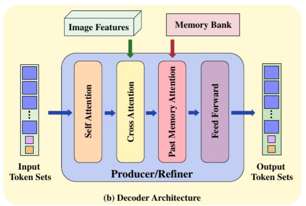
Figure 8. Architecture of a Producer/Refiner block (figure from the paper, Fig. 1b).

The Producer and the Refiner are each a single decoder block with the same design (Figure 8) but separate weights. The Producer runs once, on the learned token sets; the Refiner runs 7 times, with the same weights, on its own output.

Each block chains four sub-layers: self-attention, cross-attention, past-memory attention and a feed-forward layer.

Three attention mechanisms

The three attention layers use the same queries, the current tokens of the patch, but attend to different keys and values.

Attention works like a chest of drawers:

each key \(K\) is the label of a drawer
each value \(V\) its content
A query \(Q\) is a question compared with all the labels
The answer is a mix of the contents of the drawers whose labels match it best.

Formally :

the queries \(Q = XW_Q\) are computed from the current tokens \(X\)
the keys \(K = YW_K\) and values \(V = YW_V\) from a source \(Y\)

\(W_Q\), \(W_K\) and \(W_V\) are learned projection matrices: three linear layers, trained with the rest of the model, that turn each token into its query, key and value.

\[\text{Attention}(Q, K, V) = \text{softmax}\left(\frac{QK^\top}{\sqrt{d}}\right) V\]

\(QK^\top\) compares each question with each label, the softmax turns these scores into weights that sum to 1 (which drawers to open), and multiplying by \(V\) mixes the contents of these drawers; \(d\) is the dimension of the keys.

Attention	Source \(Y\) of the keys \(K\) and values \(V\)	Example of question \(Q\) (from a node token)	Role
Self-attention	The current tokens themselves: the 20 token sets, the past trajectory token and the step token	“Which other trajectories head toward the same branch as me, and where do we split?”	Trajectories see each other: they share out the branches between them, and read the context tokens (past trajectory, step).
Cross-attention	The image features of the current patch	“Is there a tube at my position, and in which direction does it go?”	Each token gathers the image evidence (where the tube is, its direction and width) needed to place its nodes and radii on a real branch.
Past-memory attention	The token sets stored in the memory bank, from up to 5 previous patches	“Which past nodes continue in my direction, and has this branch already been traced?”	Where the tree comes from: it keeps the direction in large vessels, where a patch only shows part of a wide tube, and reduces duplicates across patches

In short, self-attention looks within the patch’s trajectories, cross-attention looks at the image, and past-memory attention looks at the past.

Feed-forward layer

The last sub-layer is a small MLP applied to each token separately. If attention fetches the contents of the drawers, the feed-forward layer is where each token processes what it fetched: attention moves information between tokens, the feed-forward layer transforms it within each token.

Matching

Why it is needed. The 20 predictions must each be assigned one of the \(m < 20\) true branches before computing a loss. The assignment is done with the Hungarian algorithm, on the L1 distance between positions and radii.

Many-to-one. DETR assigns one prediction per target and treats the others as “no object”. RefTr instead wants all 20 predictions to be useful: the targets are replicated until there are as many targets as predictions, and the Hungarian algorithm assigns one copy to each prediction (Figure 9). Each branch thus receives several predictions, spread evenly (e.g. 10 + 10 for two branches). At inference, these copies are averaged into a single branch (see the merging step), which acts as an ensemble.

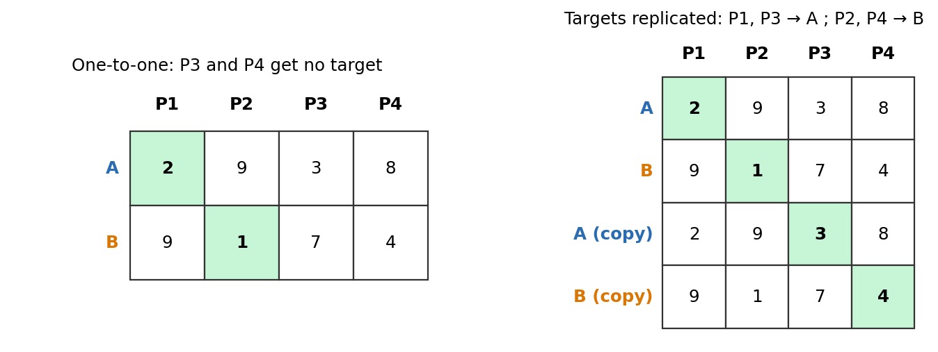
Figure 9. Many-to-one matching with 2 targets (A and B) and 4 predictions (P1 to P4). Replicating the targets lets the one-to-one Hungarian algorithm assign two predictions to each target.

Computed once. The matching is computed only once per patch on the Producer’s output (step 1), and the same assignment is kept for the 7 Refiner steps (Figure 10). The authors report that re-matching at every step destabilizes training: if a prediction could switch targets between steps, the Refiner could not learn to progressively align each trajectory with its branch.

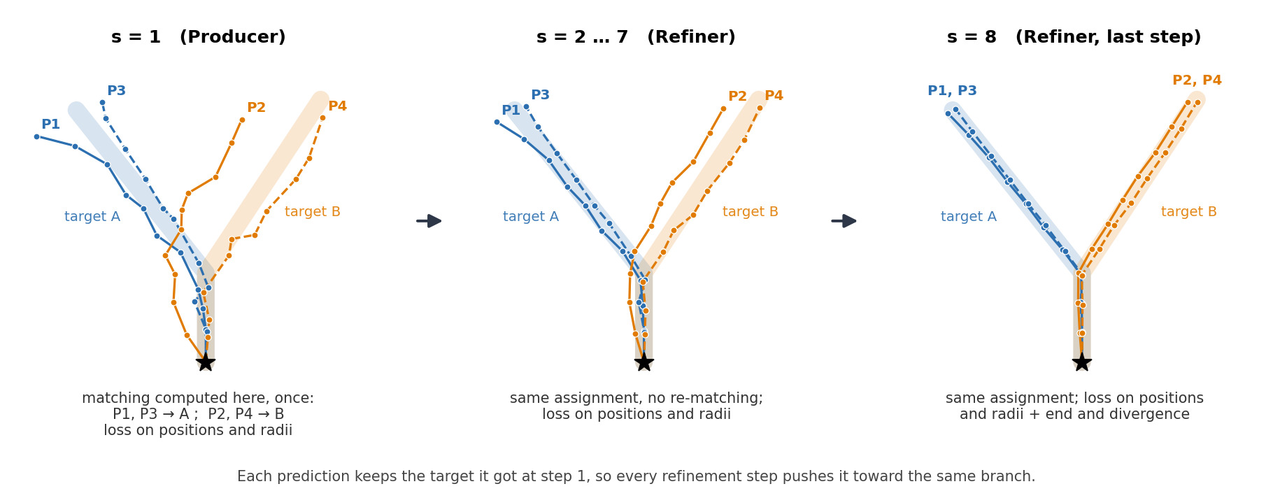
Figure 10. The matching is computed on the Producer's output and kept for all refinement steps.

The matching also gives the ground truth of the divergence head.

The Refiner steps are the same as at inference. The difference is that after every step \(s\), including the Producer step \(s = 1\), the heads decode the tokens and the predictions are compared with their matched branch :

\[\mathcal{L} = \sum_s \left( \alpha_{pos} \mathcal{L}^{(s)}_{pos} + \alpha_{rad} \mathcal{L}^{(s)}_{rad} \right) + \alpha_{end} \mathcal{L}_{end} + \alpha_{div} \mathcal{L}_{div}\]

Position and radius losses (L1) are computed at every step \(s = 1, \dots, 8\) and summed: every step, including the Producer’s proposals, is pushed toward the target.
End and divergence losses (L1) are only computed at the last step, where the trajectories are most refined.
The weights \(\alpha_{pos}=4.2\), \(\alpha_{rad}=1.2\), \(\alpha_{end}=0.9\) and \(\alpha_{div}=0.3\) were tuned on the validation split.

What is learnt

Everything is trained jointly, from scratch, with this single loss:

the image encoder (a modified SwinUNETR): features describing the tubes in the patch;
the 20 learned token sets: a generic, image-independent “identity card” of what a trajectory is, the starting point of the Producer;
the encodings of the past trajectory and of the step number;
the Producer: turning these identity cards into proposals adapted to the image and to the context;
the Refiner: a single correction, applied 7 times, that moves a set of trajectories closer to the branches. Since it is supervised after every step, it learns to improve both rough and nearly correct trajectories;
the four heads: positions, radii, end positions and divergences. The end and divergence heads are only supervised at the last step.

Passing the context

Before moving to the next patch of the chain, the context is updated as it would be at inference:

the past trajectory of the next patch is taken from the annotation;
the refined token set of the trajectory leading to the next patch is pushed into the memory bank. Only one token set is stored per patch, and the bank works as a queue of up to 5 entries: the newest is added in front and the oldest is dropped.

The next patch then starts again from the prediction step, with a new matching.

Data

The authors use three datasets, with the centerline ground truth and splits released with Trexplorer Super²:

Dataset	Structure	Images	Train / val / test
Synthetic	Vessel trees	Synthetic 3D volumes, trees generated with the Synthetic Vascular Toolkit (SVT)⁸	368 / 32 / 100
ATM’22	Airways	Chest CT	220 / 16 / 60
Parse 2022	Pulmonary arteries	CT pulmonary angiography (CTPA)	72 / 8 / 20

For the real datasets, the centerlines were extracted from the challenges’ segmentation masks, after resampling the volumes to 0.5 mm isotropic resolution.

Evaluation metrics

The authors extend the evaluation of Trexplorer Super with radius-aware matching tolerances (their third contribution). A predicted node is a true positive if it lies within

\[\delta = \max(1.5,\ \tau_{rad} \cdot r)\]

of a ground-truth node that has not been matched yet, where \(r\) is the ground-truth radius at that node. Since each ground-truth node can only be matched once, duplicates count as false positives (Figure 11a).

The tolerance factor \(\tau_{rad}\) is varied from 0.25 to 0.75 (step 0.05), and the metrics are averaged over these values, so that the results do not depend on one arbitrary tolerance.

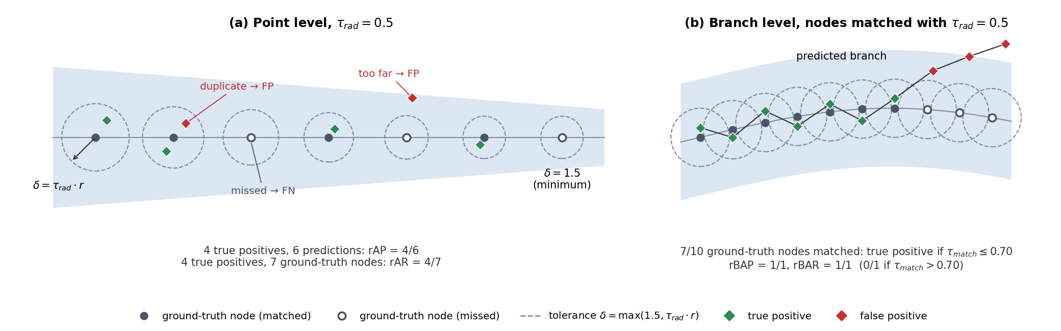
Figure 11. Radius-aware matching (toy example, not to scale). (a) Point level: true positives, false positives (too far or duplicate) and missed nodes. (b) Branch level: a branch is found if enough of its nodes are matched.

Point level, averaged over \(\tau_{rad} \in \{0.25, 0.30, \dots, 0.75\}\):

rAP (radius-aware average precision): fraction of the predicted nodes that are true positives.
rAR (radius-aware average recall): fraction of the ground-truth nodes that are matched.
rF1: F1 score, the harmonic mean of precision and recall.
Radius MAE: mean absolute error between predicted and ground-truth radii, on matched nodes.

Branch level, with nodes matched at \(\tau_{rad} = 0.5\): a predicted branch is a true positive if it covers at least a fraction \(\tau_{match}\) of the nodes of a ground-truth branch not matched yet (Figure 11b). The metrics are averaged over \(\tau_{match} \in \{0.40, 0.45, \dots, 0.80\}\):

rBAP: fraction of the predicted branches that are true positives.
rBAR: fraction of the ground-truth branches that are found.
rBF1: F1 score at branch level.

Every branch counts the same, whatever its length.

Graph level:

Betti-0 error: absolute error on the number of connected components.
Betti-1 error: absolute error on the number of cycles.

A valid tree has one component and no cycle, so both errors are zero for a valid prediction.

“Average” here means averaged over thresholds: the model outputs no confidence score, so there is no precision–recall curve as in object detection. The authors report that their conclusions are unchanged with the previous fixed thresholds.

Results

The authors run three kinds of experiments: a comparison with the state of the art, an efficiency comparison, and an ablation study. All metrics are the radius-aware metrics described above.

Comparison with the state of the art

RefTr is compared with Vesselformer (graph-based), Trexplorer and Trexplorer Super (tracking) on the three datasets. All baselines are retrained from scratch on the same splits. Results are the mean ± standard deviation over five runs, at point, branch and graph levels (full results in Tables 1 and 2 of the paper). F1 scores of the two best methods:

Dataset	Point rF1 (%), Trexplorer Super	Point rF1 (%), RefTr	Branch rBF1 (%), Trexplorer Super	Branch rBF1 (%), RefTr
Synthetic	77.98 ± 1.90	85.69 ± 1.30	78.22 ± 1.78	86.76 ± 1.38
ATM’22	61.45 ± 1.23	68.15 ± 0.59	59.87 ± 1.39	64.23 ± 0.89
Parse 2022	40.01 ± 3.86	42.37 ± 1.13	38.17 ± 3.63	37.09 ± 1.16

Conclusions.

Point level: RefTr has the best precision and recall on all three datasets. The gain is clear on Synthetic and ATM’22 (e.g. recall 66.73 % vs 60.84 % on ATM’22), but marginal on Parse 2022 (precision 53.68 % vs 53.65 %, recall 36.69 % vs 35.91 %).
Branch level: RefTr is the best on Synthetic and ATM’22, but slightly below Trexplorer Super on Parse 2022. The authors attribute this to small branches missing from the Parse ground truth: RefTr finds them (as checked by a radiologist) but they count as false positives, and every branch weighs the same regardless of its size. The small training set (72 volumes) is the other reason given.
Radius: the radius error of RefTr is higher than Trexplorer Super’s on all datasets (e.g. 0.60 vs 0.40 on ATM’22), but stays below one voxel.
Topology: all tracking methods, RefTr included, produce valid trees (zero Betti errors), whereas Vesselformer produces hundreds of extra components and cycles on the real datasets.
Qualitatively (Figure 12), RefTr captures branches that Trexplorer Super misses.

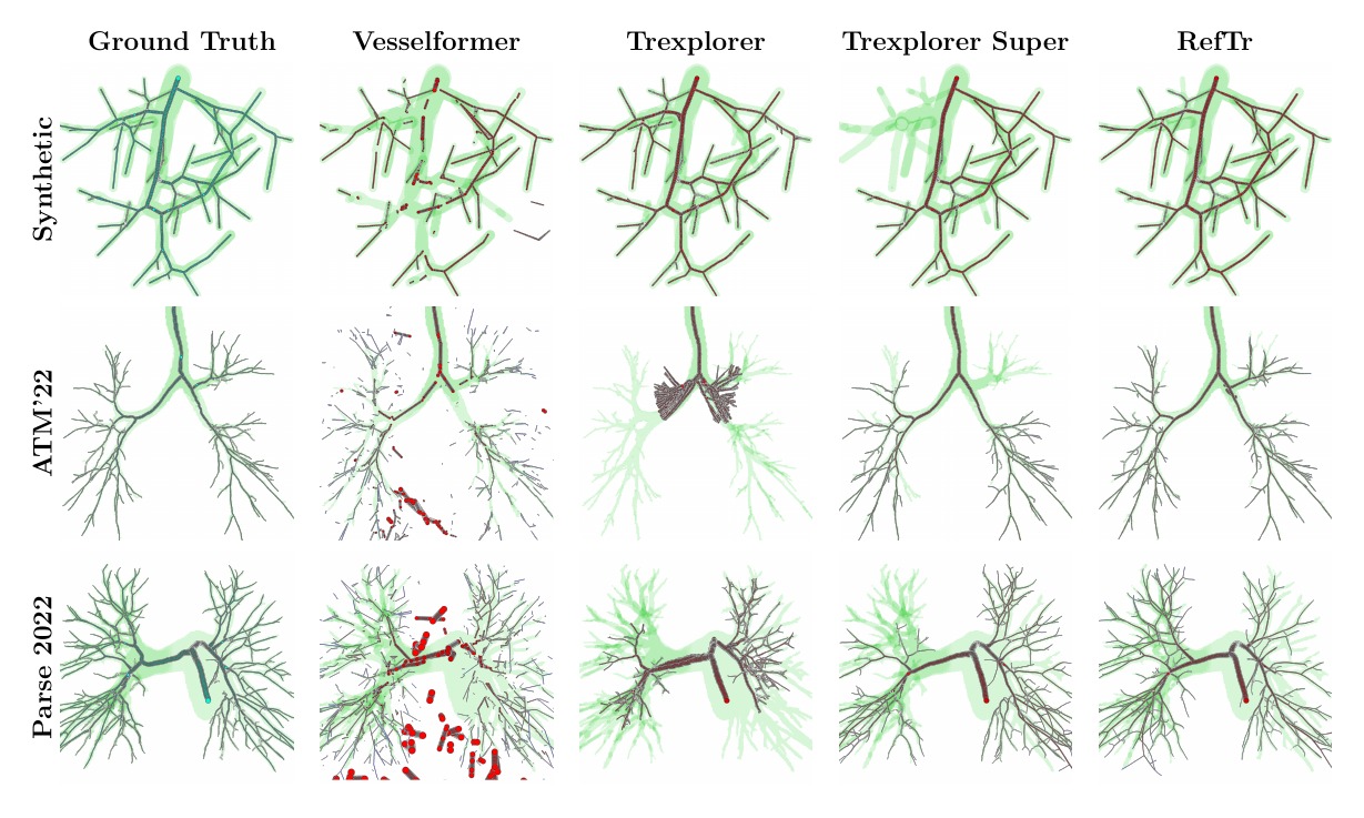
Figure 12. Qualitative comparison on one sample per dataset (figure from the paper).

Efficiency

Why. The Refiner reuses a single block for all its steps, so RefTr should be lighter than its predecessors.

How. Number of parameters, runtime per patch, training time and GPU memory, measured on four A100 80 GB GPUs (Table 3 of the paper).

Conclusions. RefTr uses the same encoder as Trexplorer Super (23.12M parameters), but its decoder is 2.4× smaller (10.50M vs 25.22M parameters). It is also faster (156 vs 189 ms per patch), trains in half the time (18.2 vs 37.2 h) and needs about half the GPU memory (39.5 vs 73.9 GB). Vesselformer is faster per patch (23 ms) but needs a multi-hour post-processing.

Ablation study

Why. To measure the contribution of each component.

How. One component is removed or changed at a time, on ATM’22, with point-level metrics averaged over three runs (Table 4 of the paper). The full model reaches rAP = 74.16 %, rAR = 67.72 % and rF1 = 68.35 %.

Conclusions.

Recurrent refinement and many-to-one matching are needed for recall. With a single Refiner step (\(S = 2\)), recall falls to 58.08 %; without many-to-one matching, to 63.25 %.
TNMS only removes duplicates. Without it, recall is unchanged (69.96 %) but precision halves (37.98 %).
8 steps is the best choice. rF1 is 58.17 %, 59.42 %, 68.35 % and 65.60 % for \(S\) = 4, 6, 8 and 10: more steps are not always better.
The past trajectory finds branches, the memory bank avoids duplicates. Without the past trajectory token, recall collapses to 37.07 % (while precision rises to 78.85 %). Without past-memory attention, precision drops to 61.27 % while recall barely changes (66.38 %).
One block each, not shared. Sharing one block between the Producer and the Refiner lowers rF1 to 60.27 %. Two Producer blocks give 63.19 % (the proposals become too rigid for the Refiner to correct, according to the authors) and two Refiner blocks 64.46 % (the updates become too large).

Conclusions

RefTr represents a tubular tree as confluent trajectories, which guarantees a valid topology, and predicts them with a Producer followed by a recurrent, weight-shared Refiner. Combined with many-to-one matching and TNMS, it improves recall and precision over the previous state of the art on three datasets, while being lighter and faster to train. The authors’ future work focuses on a better image encoder.

Remarks

What is new and what is inherited. Many components come from Trexplorer Super, by the same group:
the past trajectory token,
training on chains of 6 patches (“Super Trajectory Training”),
the focal cross-attention on a small feature crop,
the encoder,
the datasets and the evaluation framework.

The core novelty is the confluent trajectory representation with the Producer–Refiner recurrence. TNMS and the radius-aware metrics are useful but secondary contributions.

TNMS and baselines. The paper does not say whether TNMS was also applied to the baselines. Given its impact on precision in the ablation, this matters for the comparison.
Results nuance. On the real datasets, the gain over Trexplorer Super is clear on ATM’22, but small and mixed on Parse 2022, and the radius error is higher on all datasets. The strongest practical argument for RefTr is rather its efficiency: it halves the training time (18.2 vs 37.2 h) and the GPU memory (39.5 vs 73.9 GB), with a 2.4× smaller decoder.

How this post was written

This review was written with the help of an AI assistant, used as an agent that could read the paper and the code, run commands and edit the post. I want to be transparent about how, and to encourage students to use such tools openly and in a way that makes them learn rather than outsource their understanding.

What I did. First, I read the paper ;). Before asking for any draft, I used the assistant to better understand the article, asking about the parts I found unclear. Then I prompted for a first draft with the outline I wanted. From there, we refined the draft together: I chose what to keep, rewrote sections in my own way, and validated every claim. Above all, I used the assistant as a tutor: I asked “why” each time something was unclear (why the matching is computed only once, what exactly is learned in the trajectory tokens, what the keys and values of each attention layer are…) until I could explain it myself, and I challenged its answers.
What the assistant did. Set up the blog environment, read the paper and the official code, proposed a first structure and draft, created most of the figures, checked numbers and claims against the paper and the code, and pointed out inconsistencies.
What I learned from doing it this way. The draft was a starting point, not the result. Several statements were imprecise or went beyond what the paper says, and figures needed corrections. They were caught because I questioned them and went back to the paper. The writing also needed work: some sentences were convoluted or redundant, and the level of detail was not always the one I wanted, so I asked for simpler formulations or rewrote them myself.

All remaining errors and all opinions are mine. If you use an AI assistant for a review, use it to understand the paper, not to avoid reading it: ask questions, ask for sources, and check them.

References

R. Naeem et al. Trexplorer: Recurrent DETR for topologically correct tree centerline tracking. MICCAI 2024. ↩ ↩²
R. Naeem et al. Trexplorer Super: Topologically correct centerline tree tracking of tubular objects in CT volumes. MICCAI 2025. arXiv ↩ ↩² ↩³
S. Shit et al. clDice - a novel topology-preserving loss function for tubular structure segmentation. CVPR 2021. ↩
G. Tetteh et al. DeepVesselNet: Vessel segmentation, centerline prediction, and bifurcation detection in 3-D angiographic volumes. Frontiers in Neuroscience 2020. ↩
S. Shit et al. Relationformer: A unified framework for image-to-graph generation. ECCV 2022. ↩
C. Prabhakar et al. Vesselformer: Towards complete 3D vessel graph generation from images. MIDL 2024. ↩
R. Selvan et al. Extracting tree structures in CT data by tracking multiple statistically ranked hypotheses. Medical Physics 2019. ↩
Z. A. Sexton et al. Rapid model-guided design of organ-scale synthetic vasculature for biomanufacturing. arXiv preprint 2023. Code ↩

RefTr: Recurrent Refinement of Confluent Trajectories for 3D Tubular Tree Centerlines

Highlights

Introduction

Inference

Prediction and refinement

Producer

Trajectory representation

Context tokens

Refiner

Memory Bank

Prediction heads

Divergence index

Merging trajectories and building the tree

Tree Non-Maximum Suppression (TNMS)

Training

Input: 6 consecutive patches

Prediction

Producer and Refiner blocks

Three attention mechanisms

Feed-forward layer

Matching

Refinement and loss

What is learnt

Passing the context

Data

Evaluation metrics

Results

Comparison with the state of the art

Efficiency

Ablation study

Conclusions

Remarks

How this post was written

References