The beauty of contrastive learning: a new step toward efficient unsupervised learning
Notes
- Here is a link to an interesting video to better understand the contrastive learning paradigm: video
Introduction
The goal of the unsupervised model is to learn effective representation without human supervision. Most mainstream approaches can be divided into two classes: generative or discriminative.
Generative approaches learn to generate samples in the input space, such as GAN [1].
Discriminative approaches learn representation by performing pretext tasks where both the input and label are derived from an unlabeled dataset [2].
Recently, the discriminative approach based on contrastive learning in the latent space has shown great promise and achieved state-of-the-art results. The purpose of this tutorial is to introduce the key steps/concepts of this formalism, as well as the results obtained.
SimCLR framework
To understand the contrastive learning mechanism, we will start by looking at the simple contrastive learning framework for visual representation, called SimCLR. The corresponding architecture is given below:
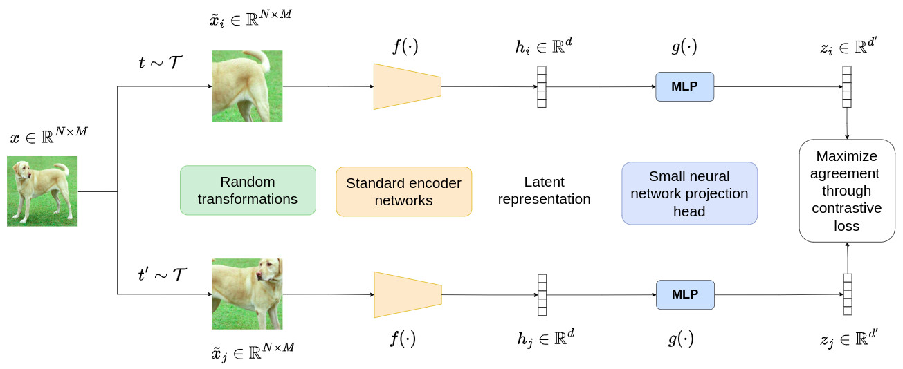
Overall scheme
As illustrated in the figure above, SimCLR comprises four major components:
-
A stochastic data augmentation module that randomly transforms any given data sample \(x\), resulting in two correlated views of the same sample, denoted as \(\tilde{x}_i\) and \(\tilde{x}_j\). These views are considered as a positive pair. The transformation applied here is the combination of random cropping, random color distortions, and random Gaussian blur.
-
A neural-network-based encoder \(f(\cdot)\) that extracts the representation vectors from the augmented data samples. This step can be realized by any standard network architecture, such as ResNet. The step is modeled as follows:
where \(h_i \in \mathbb{R}^{d}\) is the output vector after the average pooling layer.
-
A simple neural network projection head \(g(\cdot)\) that maps the representations to the space where the contrastive loss is applied. A simple MLP with one hidden layer is used in this step to output a vector \(z_i \in \mathbb{R}^{d'}\) with \(d'=128\). This allows to project the representation to a 128-dimensional latent space.
-
A contrastive loss function defined for a contrastive prediction task. Given a set of \(\{\tilde{x}_k\}\) including a positive pair of samples \(\tilde{x}_i\) and \(\tilde{x}_j\), the contrastive prediction task aims to identify \(\tilde{x}_j\) in \(\{\tilde{x}_k\}_{k \neq i}\) for a given \(\tilde{x}_i\).
Contrastive loss
-
A minibatch of \(N\) samples is randomly selected.
-
Each sample is used to create a pair of augmented examples, resulting in \(2N\) data points.
-
For each minibatch, one pair is considered as positive and the others \(2(N-1)\) as negative examples.
-
The cosine similarity between two samples \(u\) and \(v\) is computed from the conventional dot product \(sim(u,v)=u^{T}v/\left(\|u\|\|v\|\right)\). The corresponding value varies between -1 (when \(u\) and \(v\) are opposite) and 1 (when \(u\) and \(v\) are aligned).
-
The loss function for a positive pair of samples \((i,j)\) is defined as:
where \(\mathbb{1}_{[k \neq i]} \in [0,1]\) is an indicator function that outputs 1 if \(k \neq i\) while \(\tau\) is a parameter.
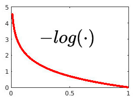
Since both the numerator and denominator involve exponential terms, the values inside the \(-\log(\cdot)\) function vary between 0 and 1. As a reminder, the corresponding curve is plotted right below. This curve shows that the loss function tends to its minimum when the numerator and the denominator are close. This means the set \(\{\exp\left(sim(z_i,z_k)/\tau\right)\}_{[k \neq (i,j)]}\) is as low as possible and \(\exp\left(sim(z_i,z_j)/\tau\right)\) is high, making the two points \(z_i\) and \(z_j\) to be as close as possible while the other points should be as far away as possible to these two points. Thus, the minimization of the contrastive loss allows the structuring of the latent space according to the visual representation!
- The final loss is computed across all positive pairs, both \((i,j)\) and \((j,i)\), in a mini-batch as follows:
Training tricks
-
The model was trained with a batch size, N=4096 for 100 epochs.
-
The training was stabilized thanks to the use of the LARS optimizer.
-
The model was trained with 128 TPU v3 cores.
-
It took around 1.5 hours to train a SimCRL model that composed of a ResNet-50 with the configurations mentionned before.
Highlights and results
- SimCRL achieved comparable results to those of supervised methods but with much more parameters to train !

-
A composition of data augmentation operations (in particular random cropping and random color distortion ) is crucial for learning good representations.
-
Unsupervised contrastive learning benefits more from bigger models than its suerpvised counterpart.
-
A nonlinear projection head improves the representation quality of the layer before it!
-
Normalized cross-entropy loss with adjustable temperature works better than its alternatives.
-
Contrastive learning benefits (more) from larger batch sizes and longer training epochs.
