Introduction to Normalizing Flows
Note
The review is not focused on a single article; the idea is to introduce a type of models, Normalizing Flows, by presenting some articles that have proposed the main advances on this field. The references of all these articles are reported at the end of the page.
This video may help understanding better this topic.
This paper is at the basis of this review:
- George Papamakarios, Eric Nalisnick, Danilo Jimenez Rezende, Shakir Mohamed, Balaji Lakshminarayanan, “Normalizing Flows for Probabilistic Modeling and Inference”, Journal of Machine Learning Research 2022.
Highlights
- Normalizing flow is a method to construct complex distributions by transforming a probability density by applying a sequence of simple invertible transformation functions.
- Flow-based generative models are fully tractable, allowing exact likelihood computation and both easy sample generation and density estimation.
- Normalizing flows have multiple applications including data generation, density estimation for outlier detection, noise modelling, etc.
Introduction
Motivation
Main generative models include Generative Adversarial Network and Variational Auto-Encoder, that have both demonstrated impressive performance results on many tasks. However, these models have several issues limiting their application, one of them being that they do not allow for exact evaluation of the density of new points. Normalizing flow are a family of generative model with tractable distributions where both sampling and density evaluation can be efficient and exact.
Change of variable
Let \(x \in X\) be a random variable with a density function \(p_{X}\) and denote \(f : X \to Z\) a diffeomorphism. The change of variable operated by \(f\) can be used to transform \(z \sim p_{Z}(z)\) into a simpler random variable \(z = f(x)\). One probability density can be retrieved from the other with the following formula :
\[p_{X}(x) = p_{Z}(f(x)) |\text{det}( \frac{\partial f(x)}{\partial x})|\]where \(\frac{\partial f}{\partial z}\) is the Jacobian matrix of the application \(f\) and \(\text{det}(\cdot)\) designates the determinant of a matrix.
Normalizing flow
Normalizing flow is a type of generative models made for powerful distribution approximation. It allows to transform a complex distribution into a simpler one (typically a multivariate normal distribution) though a serie of invertible mappings. As need to have a diffeomorphism restricts the choice of transformation functions, the final transformation is often constructed with a serie of simple applications \(f_1, ..., f_K\) :
\[f = f_K \circ f_{K-1} \circ \, ... \circ f_1\]During the successive modifications, a sample \(x\) from real data flows though a sequence of transformations and is progressively normalized. The following figure illustrates principle of this type of model :
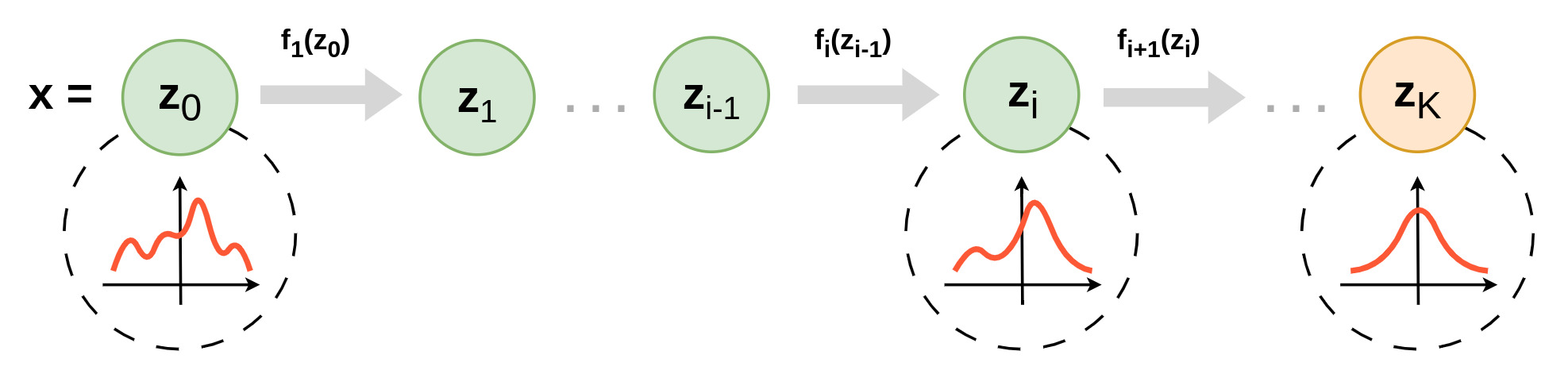
Figure 1. Illustration of a normalizing flow model.
Given such transformation, it is possible to compute directly the likelihood of some data observed \(x = \{x^{(i)}\}_{i=1,...,N}\) :
\[\log p(x;\theta, \psi) = \sum_{i=1}^{N} \log p_{Z}(f(x^{(i)};\theta) ; \psi) + \log |\text{det} \frac{\partial f(x^{(i)};\theta)}{\partial x^{(i)}} | \\ = \sum_{i=1}^{N} \log p_{Z}(f(x^{(i)};\theta);\psi) + \sum_{k=1}^{K} \log |\text{det} \frac{\partial f_{k}(x_{k-1}^{(i)};\theta_k)}{\partial x_{k-1}^{(i)}} |\]where \(\theta=(\theta_1,...,\theta_K)\) and \(\psi\) respectiveley denotes the parameters of the transformation \(f\) and the target distribution \(p_{Z}\).
Compared to other generative models such as GANs or VAEs, the optimization problem is much more straightforward as it can be done directly via the maximization of the likelihood and does not require an adversarial network or the introduction of a lower bound of the likelihood.
Density estimation is done with the direct path of the transformation flow chain and allows to evaluate the probability of any new sample. To create new data, a sample \(z \sim p_{Z}(z)\) is generated from the simple distribution and flows though the backwards pass of the chain \(g = f_1^{-1} \circ \, ... \circ f_K^{-1}\).
NOTE: Since all the functions involved in the transormation of densities are bijective and differentiable, the normalizing flow process can be equivalently introduced the other way around. The version that is shown here is more oriented towards density estimation, while presenting the reverse path first (from simple distribution to complex data) may be more suitable if the final purpose is data generation.
Types of flow
Theoretically, any diffeomorphism could be used to build a normalizing flow model, but in practice it should satisfy two properties to be applicable:
- Be invertible with an easy-to-compute inverse function (depending on the application)
- Computing the determinant of its Jacobian needs to be efficient. Typically, we want the Jacobian be a triangular matrix.
Therefore, designing flows is one of the core problem adressed by research on this topic. The objective is to find functions such as described above that can still be complex enough to build models that yield good expressive power.
Illustration with planar and radial flows
In the change of variable formula, the absolute value of the determinant of the jacobian of \(f\) is a dilation/retractation factor of the space. In low dimension and with simple transformation function, it is possible to observe how an initial density function can be distorted during the flow process.
We consider famiily of transformations, called planar flows1, described by:
\[f(\textbf{z}) = \textbf{z} + \textbf{u}h(\textbf{w}^{T}\textbf{z} + b)\]where \(\lambda = \{\textbf{w} \in \mathbb{R}^{D}, \textbf{u} \in \mathbb{R}^{D}, b \in \mathbb{R} \}\) are free parameters and \(h(\cdot)\) is a differentiable element-wise and non-linear function. This particular flow transforms a density by applying a series of contractions and expansions in the direction perpendicular to the hyperplane \(\textbf{w}^T \textbf{z}+b = 0\). For this mapping, we can compute the determinant of the Jacobian in \(O(D)\) time :
\[| \text{det} \frac{\partial f}{\partial z} | = |1+\textbf{u}^Th'(\textbf{w}^{T}\textbf{z} + b)\textbf{w} |\]
Similarly, the family described by :
\[f(\textbf{z}) = \textbf{z} + \beta h(\alpha,r)(\textbf{z} - \textbf{z}_0)\] \[| \text{det} \frac{\partial f}{\partial z} | = [1+\beta h(\alpha,r)]^{d-1} [1+\beta h(\alpha,r)+\beta h'(\alpha,r)r ]\]with \(r = |\textbf{z} - \textbf{z}_0|\), \(h(\alpha,r)=1/(\alpha + r)\), and parameters \(\lambda= \{ \textbf{z}_0 \in \mathbb{R}^D, \alpha \in \mathbb{R}^{+}, \beta \in \mathbb{R} \}\), applies contractions and expansions around the reference point \(\textbf{z}_0\) and is called radial flow.
The effect of these types of transformations can be seen in Fig. 2 for two examples of 2D distributions.
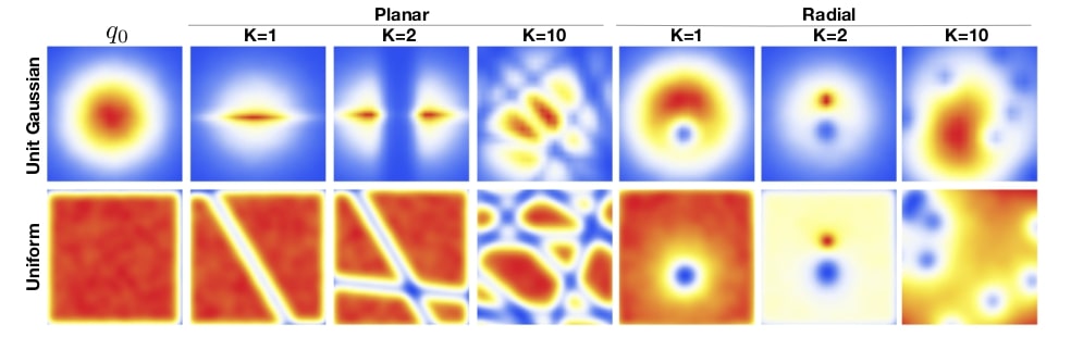
Figure 2. Effect of planar and radial flow on two distributions1.
Coupling layers
A core family of transformation has been introduced by Dinh et al.2 in 2015 and is called coupling layers.
An input vector \(z\) is split into \(z_{1:d}\) and \(z_{d+1:D}\). In the forward pass, the ouput vector \(x\) is obtained as follows (Fig. 3) :
\[\left\{ \begin{array}{ll} x_{1:d} = z_{1:d} \\ x_{d+1:D} = g(z_{d+1:D},m(z_{1:d})) \end{array} \right.\]where \(m(\cdot)\) can by any function and \(g(\cdot)\) is an invertible function. If \(g\) is easy enough to invert, the backwards pass is simple as well :
\[\left\{ \begin{array}{ll} z_{1:d} = x_{1:d} \\ z_{d+1:D} = g^{-1}(x_{d+1:D},m(x_{1:d})) \end{array} \right.\]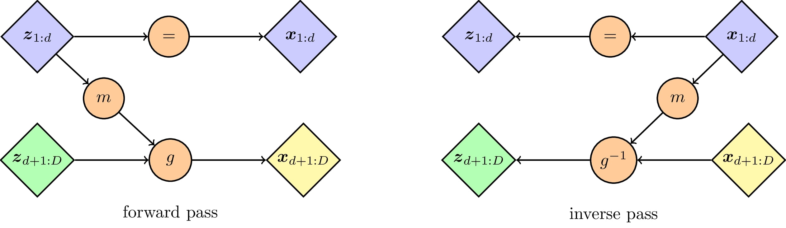
Figure 3. Illustration of the principle of coupling layers.
The Jacobian matrix of this transformation is :
\[\frac{\partial x}{\partial z} = \begin{bmatrix} \textbf{I}_d & 0\\ \frac{\partial x_{d+1:D}}{\partial z_{1:d}} & \frac{\partial x_{d+1:D}}{\partial z_{d+1:D}} \end{bmatrix}\]The key of this flow is that there is no need to invert the mapping \(m(\cdot)\) to compute the determinant of the Jacobian, thus it can be anything, such as a dense neural network, a CNN, a Transformer, etc. Only the function \(g(\cdot)\) needs to remain relatively simple, for instance affine with non-linear scaling factors.
Since only a fraction of the input vector goes though a complex transformation, coupling layers are stacked and alternated with permutations 3 to improve the expressivity of the flow model.
Examples of results
In 2016, Dinh et al. 3 introduced Real NVP, a flow model using real-valued non-volume preserving transformations. It was one of the first deep learning model using normalizing flow to perform density estimation and image generation. The results with this model, shown in Fig. 4, are far from the standards we have now but is similar to the best generative models at that time.
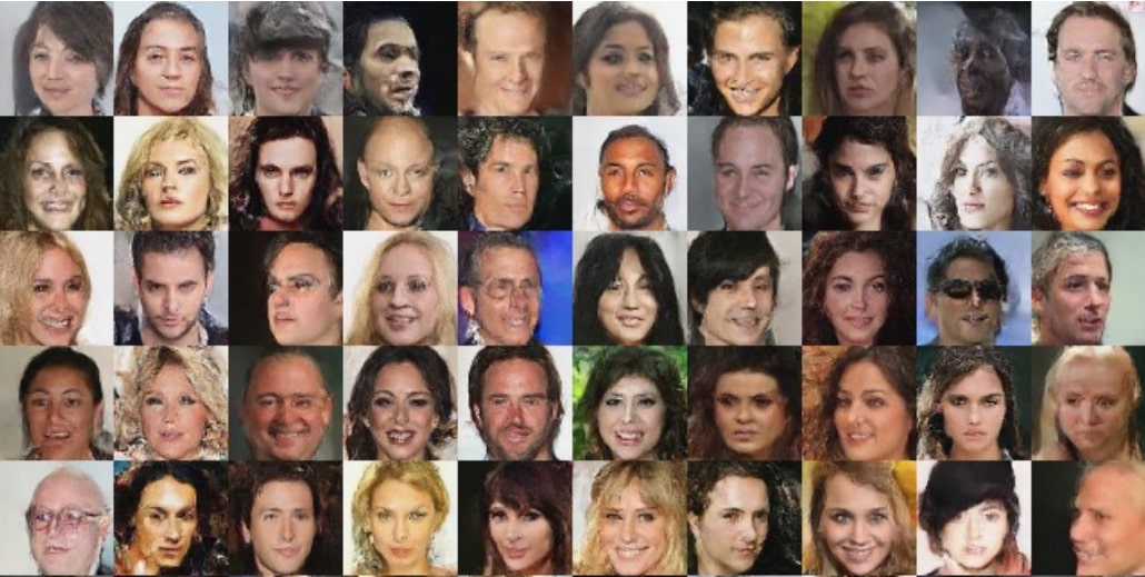
Figure 4. Examples of faces generated by Real NVP trained on CelebFaces Attributes dataset.
Later, in 2018, Glow4 used coupling layers and introduced 1x1 invertible convolutions to achieve much better looking results are set a new state-of-the-art flow-based generative model.
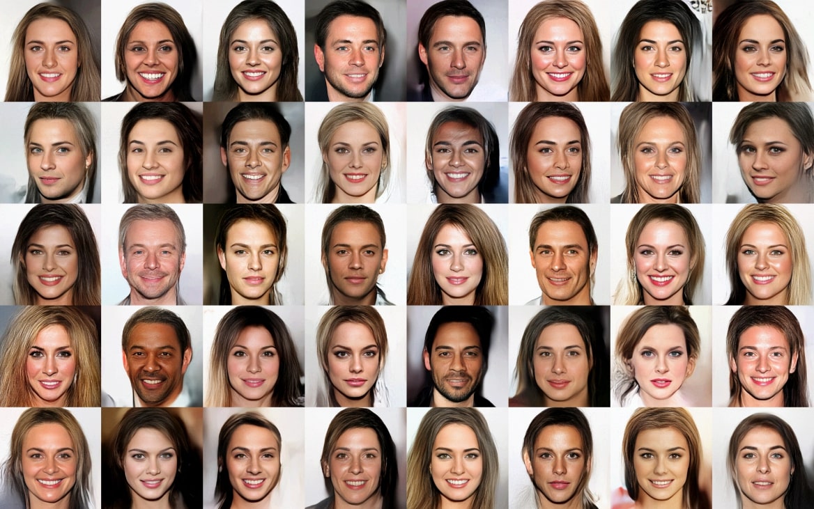
Figure 5. Examples of faces generated by GLOW trained on CelebFaces Attributes dataset.
For several years now, flow models are used to performed diverse tasks such as unsupervised anomaly detection. With FastFlow5 for example, Wu. et al. achieved state-of-the-art performances on the task of unsupervised anomaly detection on the industrial dataset MVTec AD.
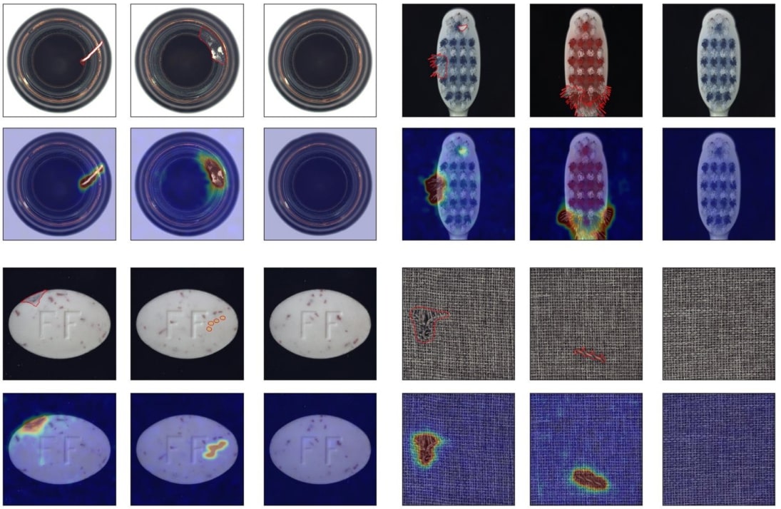
Figure 6. Examples of unsupervised anomaly detection on an industrial dataset using normalizing flow.
Conclusion
Flow models are a type a generative models designed to transform distributions in fully tractable way though a series a invertible mappings. They can be used for many application related to data generation and density estimation.
References
-
D. Jimenez Rezende, S. Mohamed. Variational Inference with Normalizing Flows. June 2016. ↩
-
L. Dinh, D. Krueger, Y. Bengio. NICE: Non-linear Independent Components Estimation. In ICLR. April 2015. ↩
-
L. Dinh, J. Sohl-Dickstein and S. Bengio. Density estimation using Real NVP. In ICLR. February 2017. ↩ ↩2
-
D. P. Kingma, P. Dhariwal. Glow: Generative Flow with Invertible 1x1 Convolutions. July 2018. ↩
-
J. Wu et al. FastFlow: Unsupervised Anomaly Detection and Localization via 2D Normalizing Flows. November 2018. ↩