The denoising diffusion probabilistic models (DDPM) paradigm demystified
Notes
-
Here are links to two video and an excellent post that we used to create this tutorial: video1, video2, post.
- Introduction
- Fondamental concepts
- Forward diffusion process
- Reverse process
- To go further
Introduction
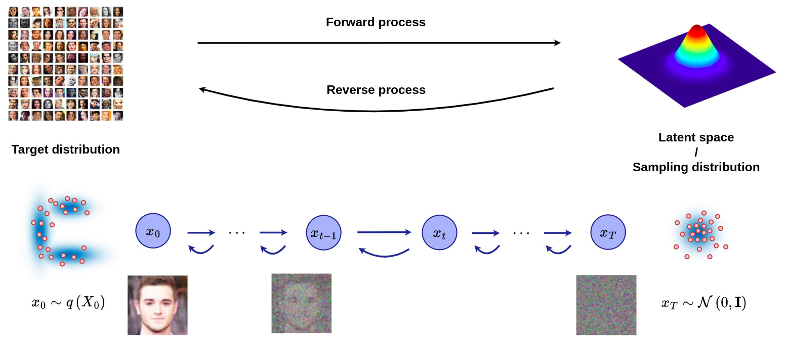
Overview of diffusion models (DM)
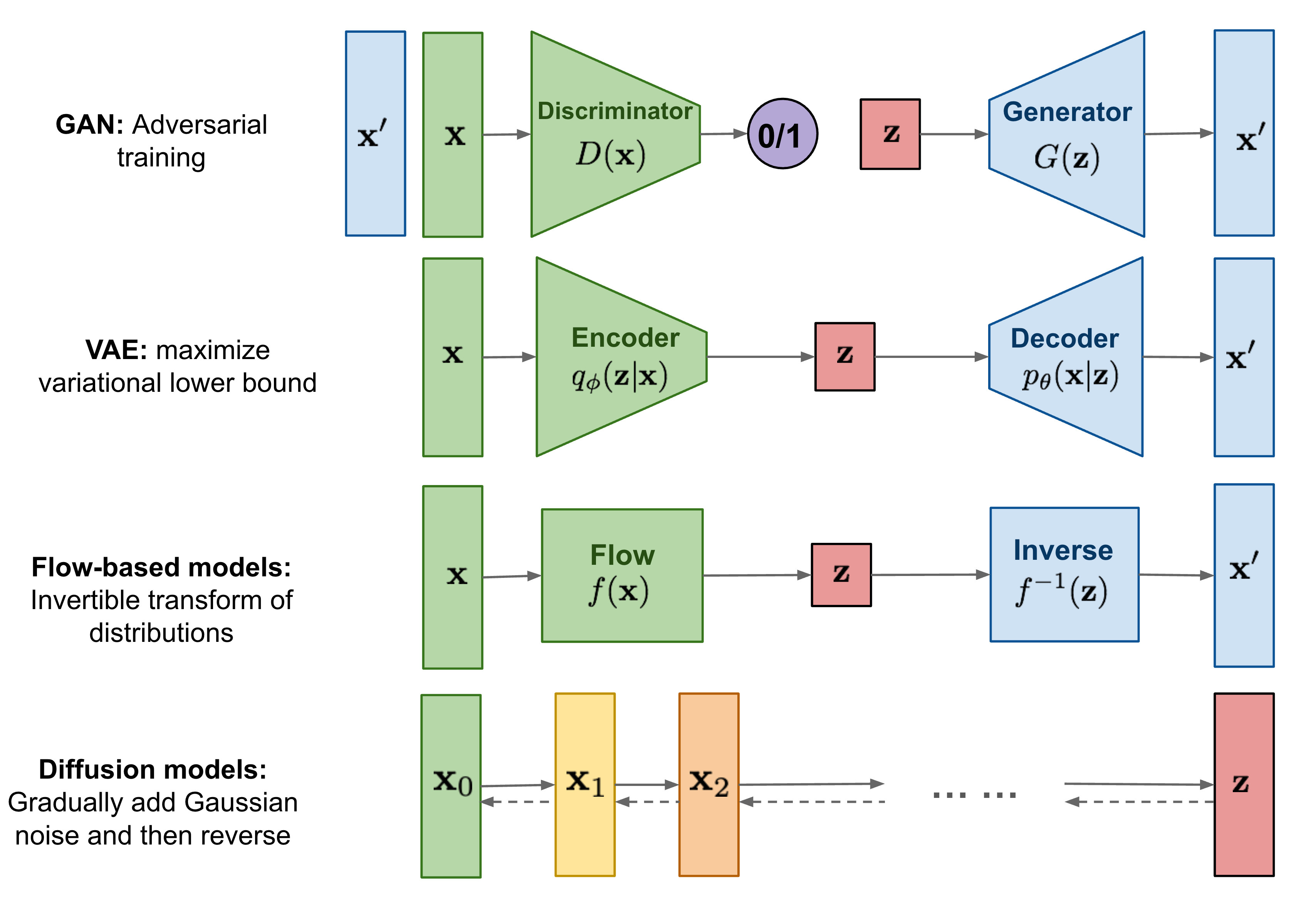
- DM are a class of generative models such as GAN, normalizing flow or variational auto-encoders.
- DM define a Markov chain of diffusion steps to slowly add random noise to data.
- The model then learns to reverse the diffusion process to construct data samples from noise.
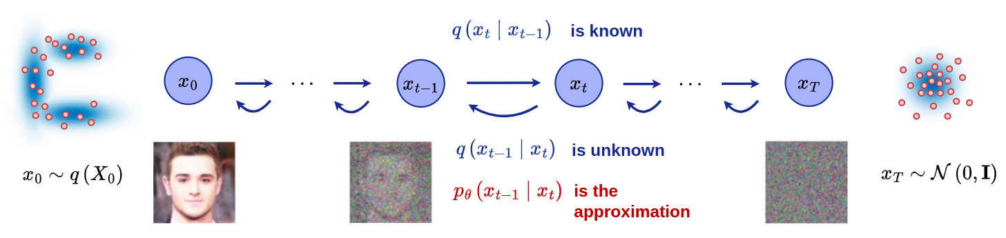
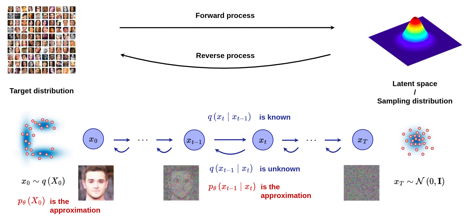
- The figure below gives an overview of the Markov chain involved in the DM formalism, where the forward (reverse) diffusion process is the key element in generating a sample by slowly adding (removing) noise.
Diffusion models vs generative models
- DM belong to the generative models family.
- DM have demonstrated effectiveness in generating high-quality samples.
- Unlike GAN, VAEs and flow-based models, the latent space involved in the DM formalism has high-dimensionality corresponding to the dimensionality of the original data.
- The figure below gives and overview of the different types of generative models:
Fondamental concepts
Sum of normally distributed variables
- If \(x\) and \(y\) be independent random variables that are normally distributed \(x \sim \mathcal{N}(\mu _X , \sigma ^2_X \, \mathbf{I})\) and \(y \sim \mathcal{N}(\mu _Y , \sigma ^2_Y \, \mathbf{I})\) then \(x + y \sim \mathcal{N}(\mu _X + \mu _Y, (\sigma ^2_X + \sigma ^2_Y) \, \mathbf{I})\)
The sum of two independent normally distributed random variables is also normally distributed, with its mean being the sum of the two means, and its variance being the sum of the two variances.
-
If \(x \sim \mathcal{N}(0, \mathbf{I})\) then \(\sigma \, x \sim \mathcal{N}(0, \sigma^2 \, \mathbf{I})\).
-
If x and y be independent standard normal random variables \(x \sim \mathcal{N}(0, \mathbf{I})\) and \(y \sim \mathcal{N}(0, \mathbf{I})\), the sum \(\sigma_X x + \sigma_Y y\) is normally distributed such as \(\sigma_X x + \sigma_Y y \sim \mathcal{N}(0, (\sigma^2_X + \sigma^2_Y) \, \mathbf{I})\).
Bayes Theorem
\[q(x_{t} \mid x_{t-1}) = \frac{q(x_{t-1} \mid x_{t}) \, q(x_{t})}{q(x_{t-1})}\] \[q(x_{t-1} \mid x_t) = \frac{q(x_t \mid x_{t-1}) \, q(x_{t-1})}{q(x_t)}\]
Conditional probability theorem
\[q(x_{t-1} , x_{t}) = q(x_{t} \mid x_{t-1}) q(x_{t-1})\] \[q(x_{1:T} \mid x_0) = q(x_T \mid x_{0:T-1}) q(x_{T-1} \mid x_{0:T-2}) \dots q(x_1 \mid x_0)\]
Marginal theorem
\[q(x_{0},x_{1},\cdots,x_{T}) = q(x_{0:T})\] \[q(x_{0}) = \int q(x_{0},x_{1},\cdots,x_{T}) \,dx_{1}\,\cdots\,dx_{T}\] \[q(x_{0}) = \int q(x_{0:T}) \,dx_{1:T}\]
Markov chain properties
In a Markov chain, the probability of each event depends only on the state attained in the previous event. The following expressions can thus be written:
Conditional probability theorem
\[q(x_T \mid x_{0:T-1}) = q(x_T \mid x_{T-1})\] \[q(x_{1:T} \mid x_0) = \prod_{t=1}^{T} q(x_t \mid x_{t-1})\] \[p_{\theta}(x_{0:T}) = p_{\theta}(x_{T}) \prod_{t=1}^{T} p_{\theta}(x_{t-1} \mid x_{t})\] \[q(x_{t} \mid x_{t-1}) = q(x_{t} \mid x_{t-1}, x_0) = \frac{q(x_{t-1} \mid x_{t}, x_0) \, q(x_{t} \mid x_0)}{q(x_{t-1} \mid x_0)}\]
Reparameterization trick
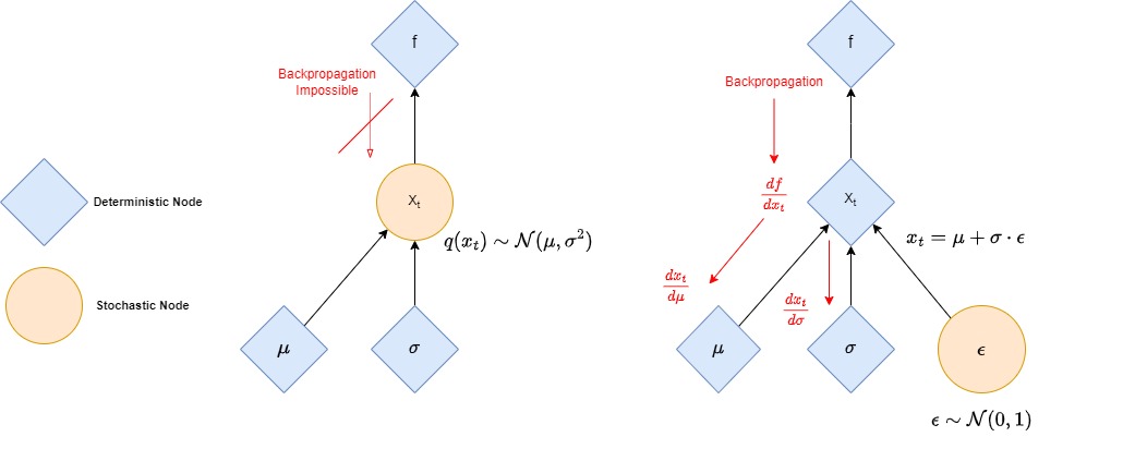
- Transform a stochastic node sampled from a parameterized distribution into a deterministic one.
- Allows backpropagation through such a stochastic node by turning it into deterministic node.
- Let’s assume that \(x_t\) is a point sampled from a parameterized Gaussian distribution \(q(x_t)\) with mean \(\mu\) and variance \(\sigma^2\).
- The following reparametrization trick uses a standard normal distribution \(\mathcal{N}(0,\mathbf{I})\) that is independent of the model, with \(\epsilon \sim \mathcal{N}(0,\mathbf{I})\):
- The prediction of \(\mu\) and \(\sigma\) is no longer tied to the stochastic sampling operation, which allows a simple backpropagation process as illustrated in the figure below
Cross entropy
- Entropy \(H(p)\) corresponds to the average information of a process defined by its corresponding distribution
Cross entropy measures the average number of bits needed to encode an event when using a different probability distribution than the true distribution.
\[H_{pq} = -\int{p(x)\cdot \log\left(q(x)\right)}\,dx = \mathbb{E}_{x \sim p} [\log(q(x))]\]
- It can also be seen as a tool to quantify the extent to which a distribution differs from a reference distribution. It is thus strongly linked to the Kullback–Leibler divergence measure as follows:
- \(H(p)\), \(H(p,q)\) and \(D_{KL}(p \parallel q)\) are always positives.
When comparing a distribution \(q\) against a fixed reference distribution \(p\), cross-entropy and KL divergence are identical up to an additive constant (since \(p\) is fixed).
Forward diffusion process
Principle
-
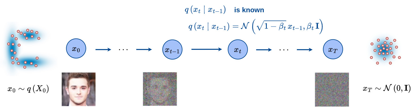
Let’s define \(x_0\) a point sampled from a real data distribution \(x_0 \sim q(X_0)\).
-
The forward diffusion process is a procedure where a small amount of Gaussian noise is added to the point sample \(x_0\), producing a sequence of noisy samples \(x_1, \cdots , x_T\).
The forward process of a probabilistic diffusion model is a Markov chain, i.e. the prediction at step \(\,t\) only depends on the state at step \(\,t-1\), that gradually adds Gaussian noise to the data \(\,x_0\).
- The full forward process can be modeled as:
- Based on the definition of the forward process, the conditional distribution \(q(x_t \mid x_{t-1})\) can be efficiently represented as:
-
The step sizes are controlled by a variance schedule \(\{ \beta_t \in [0,1] \}_{t=1}^T\)
-
\(\beta_t\) becomes increasingly larger as the sample becomes noisier, i.e.
- Based on the above equation, the two extreme cases can be easily derived:
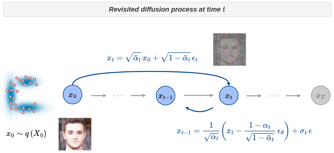
- A nice property of the forward process is that we can sample \(x_t\) at any arbitrary time step \(t\) in a closed form using reparametrization trick and the property of the sum of normally distributed variables, as shown below:
\(\quad\) Let’s define \(\alpha_t = 1 - \beta_t\)
\[x_t = \sqrt{\alpha_t} \, x_{t-1} + \sqrt {1-\alpha_t} \, \epsilon_{t-1}\]\(\quad\) This expression is true for any \(t\) so we can write
\[x_{t-1} = \sqrt{\alpha_{t-1}} \, x_{t-2} + \sqrt{1-\alpha_{t-1}} \, \epsilon_{t-2}\]\(\quad\) and
\[x_t = \sqrt{\alpha_t \alpha_{t-1}} \, x_{t-2} + \sqrt{\alpha_t- \alpha_t \alpha_{t-1}} \, \epsilon_{t-2} + \sqrt{1-\alpha_t} \, \epsilon_{t-1}\] \[x_t \sim \mathcal{N}\left(\sqrt{\alpha_t \alpha_{t-1}} \, x_{t-2}, \alpha_t- \alpha_t \alpha_{t-1} \right) + \mathcal{N}\left(0, 1-\alpha_t \right)\] \[x_t \sim \mathcal{N}\left(\sqrt{\alpha_t \alpha_{t-1}} \, x_{t-2}, \alpha_t- \alpha_t \alpha_{t-1} + 1-\alpha_t \right)\] \[x_t \sim \mathcal{N}\left(\sqrt{\alpha_t \alpha_{t-1}} \, x_{t-2}, 1 - \alpha_t \alpha_{t-1} \right)\] \[x_t = \sqrt{\alpha_t \alpha_{t-1}} \, x_{t-2} + \sqrt{1-\alpha_t \alpha_{t-1}} \, \bar{\epsilon}_{t-2}\]\(\quad\) One can repeat this process recursively until reaching an expression of \(x_t\) from \(x_0\):
\[x_t = \sqrt{\alpha_t \cdots \alpha_1} \, x_0 + \sqrt{1 - \alpha_t \cdots \alpha_1} \, \bar \epsilon _0\]\(\quad\) By defining \(\bar{\alpha}_t = \prod_{k=1}^{t}{\alpha _k}\), we finally get this final relation:
When \(\, T \rightarrow \infty\), \(\, \beta_t \rightarrow 1\), \(\, \alpha_t \rightarrow 0\), thus \(\, \bar{\alpha}_t \rightarrow 0\) and \(\, x_T \sim \mathcal{N}(0,\mathbf{I})\).
This means that \(x_T\) is equivalent to pure noise from a Gaussian distribution. We have therefore defined a forward process called a diffusion probabilistic process that slowly introduces noise into a signal.
How to define the variance scheduler?
-
The original article set the forward variances \(\{\beta_t \in (0,1) \}_{t=1}^T\) to be a sequence of linearly increasing constants.
-
Forward variances are chosen to be relatively small compared to data scaled to [-1,1]. This ensures that reverse and forward processes maintain approximately the same functionnal form.
-
More recently, a cosine scheduler has been proposed to improve results.
-
The variances \(\beta _t\) can be deducted from this definition as \(\beta_t = 1 - \frac{\bar{\alpha_t}}{\bar{\alpha_{t-1}}}\)
-
In practice \(\beta_t\) is clipped to be no larger than \(0,999\) to prevent singularities for \(t \rightarrow T\).

Reverse process
General idea
-
If we are able to reverse the diffusion process from \(q(x_{t-1} \mid x_t)\), we would be able to generate a sample \(x_0\) from a Gaussian noise input \(x_T \sim \mathcal{N}(0,\mathbf{I})\) !
-
Following the Bayes theorem and considering that \(q(x_t)\) is an unknown, one can easily see that \(q(x_{t-1} \mid x_t)\) is intractable.
It is noteworthy that the reverse conditional probability is tractable when conditioned on \(x_0\). Indeed, thanks to Bayes theorem \(\, q(x_{t-1} \mid x_t, x_0)\) = \(\frac{q(x_t \mid x_{t-1}, x_0)q(x_{t-1} \mid x_0)}{q(x_t \mid x_0)}\)=\(\frac{q(x_t \mid x_{t-1})q(x_{t-1} \mid x_0)}{q(x_t \mid x_0)}\), where all distributions are known from the forward process.
- The analytical expression of \(q(x_{t-1} \mid x_t, x_0)\) can be derived using the individual definitions of \(q(x_t \mid x_{t-1})\), \(q(x_{t-1} \mid x_0)\) and \(q(x_t \mid x_0)\), which leads to the following expression (see the blog of Lilian Wang for details on the derivation):
\(\quad\) where
-
However, if \(\beta_t\) is small enough, \(q(x_{t-1} \mid x_t)\) will also be Gaussian.
-
We will learn a model \(p_{\theta}\) to approximate these conditional probabilities in order to run the reverse diffusion process:
\(\mu _{\theta}(x_t,t)\) and \(\, \Sigma_{\theta}(x_t,t)\) depend not only on \(x_t\) but also on \(\,t\).
Loss function
- The reverse process loss function minimizes the cross-entropy between the target distribution \(q(X_0)\) and the approximated distribution \(p_{\theta}(X_0)\)
Minimizing the cross entropy between \(q(X_0)\) and \(\, p_{\theta}(X_0)\) results in the two distributions being as close as possible
- \(p_{\theta}(X_0)\) depends on \(X_1, X_2, \dots, X_T\). Thanks to the marginal theorem, the above expression can be rewritten as:
- Using the Jensen’s inequality, the above equation can be rewritten as:
- Since by definition, the Variational Lower Bound (VLB) is
\(\quad\) and since \(H(q,p_{\theta})\) is positive, minimizing \(\mathcal{L}_{VLB}\) is equivalent to minimizing \(H(q,p_{\theta})\).
- The minimization of \(\mathcal{L}_{VLB}\) can be further rewritten as the combination of several KL-divergence and entropy terms, as follows:
- Using the markov chain properties with Bayes, the above expression can be reformulated as:
- The variational lower bound can thus be rewritten as follows:
\(\quad\) where
\(\mathcal{L}_T\): Constant Term
- Since the forward variances \(\beta_t\) are fixed as constants, the approximate posterior \(q\) has no learnable parameters, so \(\mathcal{L}_T\) is a constant during training and can be ignored.
\(\mathcal{L}_0\): Reconstruction term
-
\(\mathcal{L}_0\) is the likelihood of a Gaussian distribution of the form \(\mathcal{N}(\mu _{\theta}(x_1,1),\Sigma _{\theta}(x_1,1))\)
-
\(p_{\theta}(x_0 \mid x_1)\) is computed as follows:
\(\quad\) where \(D\) is the data dimensionality and \(i\) indicates the extraction of one coordinate.
\[\delta _{+} (x) = \begin{cases} \infty & \text{if $x = 1$} \\ x + \frac{1}{255} & \text{if $x < 1$} \end{cases}\] \[\delta _{-} (x) = \begin{cases} -\infty & \text{if $x = -1$} \\ x - \frac{1}{255} & \text{if $x > -1$} \end{cases}\]- An independant discrete decoder is set to obtain the corresponding log likelihood.
\(\mathcal{L}_{t-1}\): Stepwise denoising terms
- Recall that \(p_{\theta}(x_{t-1} \vert x_t) = \mathcal{N}(\mu_{\theta}(x_t,t), \Sigma_{\theta}(x_t,t))\) and \(q(x_{t-1} \vert x_t, x_0) = \mathcal{N}(\tilde{\mu}_t(x_t,x_0), \tilde{\beta}_t \cdot \textbf{I})\),
the idea is first to focus on the mean terms and train a neural network \(\mu_{\theta}\) to predict \(\tilde{\mu}_t = \frac{1}{\sqrt{\alpha_t}} (x_t - \frac{1-\alpha_t}{\sqrt{1- \bar{\alpha}_t}} \epsilon _t)\)
Because \(x_t\) is available at training time, we can reparameterize the Gaussian noise term (a neural network) to make it predict \(\epsilon_t\) from the input \(x_t\)
- The loss term \(\mathcal{L}_t\) is revisited to minimize the difference between \(\mu_{\theta}\) and \(\tilde{\mu}\):
- Finally, the stepwise denoising terms are expressed as:
-
The authors from a seminal paper of the DDPM method proposed to fix \(\{\beta _t\}^T_{t=1}\) as constants for the sake of simplicity.
-
Instead of making \(\beta_t\) learnable, they set \(\Sigma _{\theta} (x_t ,t) = \sigma_t^2 \, \mathbf{I}\), where \(\sigma_t\) is not learned but set to \(\beta_t\) or \(\bar{\beta}_t = \frac{1 - \bar{\alpha}_{t-1}}{1-\bar{\alpha}_t}\cdot \beta_t\).
-
The stepwise denoising loss function becomes:
- They also found that simplifying the loss function by ignoring the weighting term improved the model training, making it less noisy:
Deep learning architecture
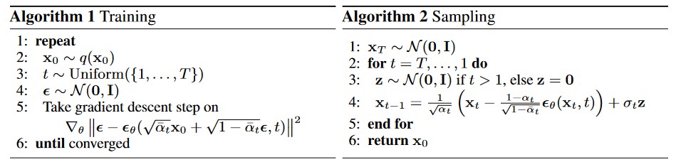
- Even if the key modeling of diffusion models is the Markov chain, it is possible to directly express \(x_t\) according to \(x_0\) using the following equation:
\(\quad\) where \(\bar{\alpha}_t = \prod_{k=1}^{t}{\alpha _k}\) and \(\alpha_t = 1 - \beta_t\).
It is thus possible to generate a random image \(\,x_t\) of the input image \(\,x_0\) at any time \(\,t\) of the diffusion process with a known noise \(\,\epsilon_t \in \mathcal{N}(0,\mathbf{I})\) from the input image.
-
For diffusion models, the deep learning architecture aims to estimate \(\epsilon_t\) from \(x_t\) at time \(t\). The estimated noise is denoted \(\epsilon_{\theta}(x_t,t)\).
-
Recall that \(p_{\theta}(x_{t-1} \vert x_t) = \mathcal{N}(\mu_{\theta}(x_t,t), \Sigma_{\theta}(x_t,t))\) with \(\mu_{\theta}(x_t,t) = \frac{1}{\sqrt{\alpha_t}} \left(x_t - \frac{1-\alpha_t}{\sqrt{1- \bar{\alpha}_t}}\epsilon_{\theta}(x_t,t)\right)\).
-
Making the assumption that \(\Sigma_{\theta}(x_t,t)\) is equal to \(\sigma^2_t \, \mathbf{I}\) (see previous section), the above expression can be rewritten as:
\(\quad\) where
\[\epsilon \sim \mathcal{N}(0,\mathbf{I})\]
It is thus possible for any time \(t\) to generate the corresponding noisy image \(\,x_t\) from \(\,x_0\) as well as the additional noise \(\,\epsilon_t\) and learn to estimate it from \(\,x_t\) and \(\,t\). The estimated noise \(\,\epsilon_{\theta}(x_t,t)\) can then be used to retrieve \(\,x_{t-1}\) from \(\,x_t\) as illustrated in the figure below.
-
This diffusion process can be efficiently learned using the above deep learning architecture for any time \(t\) and for any image \(x_0 \sim q(X_0)\) of the targeted distribution.
-
This architecture involves a standard U-Net model with attention layers and positional embedding to encode the temporal information. This is needed as the amount of noise added varies over time.


-
During the reverse process, the set of samples \(x_T, x_{T-1}, \cdots, x_{0}\) have to be computed in a recursive manner.
-
Starting from \(x_T \sim \mathcal{N}(0,\mathbf{I})\) and keeping in mind that \(p_{\theta}(x_{t-1} \mid x_t) = \mathcal{N}\left( \mu_{\theta}(x_t,t), \Sigma_{\theta}(x_t,t) \right)\) this is done through the following relation:
To go further
Parameterization of reverse process variance
- In a recent article, the authors proposed to improve DDPM results by learning \(\Sigma _{\theta}(x_t,t)\) as an interpolation between \(\beta_t\) and \(\bar{\beta}_t\) by predicting a mixing vector \(\mathbf{v}\):
- Since \(\mathcal{L}_{simple}\) does not depend on \(\Sigma_{\theta}(x_t,t)\), the following new hybrid loss function was defined:
- \(\lambda = 0.001\) to prevent \(\mathcal{L}_{VLB}\) from dominating \(\mathcal{L}_{simple}\) and applied a stop gradient on \(\mu_{\theta}(x_t,t)\) in the \(\mathcal{L}_{VLB}\) term such that \(\mathcal{L}_{VLB}\) only guides the learning of \(\Sigma_{\theta}(x_t,t)\).
The use of a time-averaging smoothed version of \(\mathcal{L}_{VLB}\) was key to stabilize the optimization of \(\mathcal{L}_{VLB}\) due to the presence of noisy gradients coming from this term.
Improve sampling speed
-
It is very slow to generate a sample from DDPM by following the Markov chain of the reverse process as \(T\) can be up to one or a few thousand steps
-
Producing a single sample takes several minutes on a modern GPU.
-
One simple way to improve this is to run a strided sampling scheduler.
-
For a model trained with \(T\) diffusion steps, the sampling procedure only use \([T/S]\) steps to reduce the process from \(T\) to \(S\) steps.
-
The new sampling schedule for data generation is \(\{\tau_1,\cdots,\tau_S\}\) where \(\tau_1 < \tau_2 < \cdots < \tau_S \in [1,T]\) and \(S<T\).
-
Another algorithm, DDIM named Denoising Diffusion Implicit Model, modifies the forward diffusion process making it non-Markovian to speed up the generation. The key is to change the forward diffusion into a non-Markovian process while keeping the reverse process Markovian but with fewer steps.
-
DDIMs defined a family of inference distributions, indexed by a real vector \(\sigma \in \mathbb{R}^{L}_{\geq 0}\) such as :
And for all t > 1 :
\[q_{\sigma}(x_{t-1} \mid x_{t}, x_{0}) = \mathcal{N}\left( \sqrt{\bar{\alpha}_{t-1}} \, x_0 + \sqrt{1 - \bar{\alpha}_{t-1} - \sigma_{t}^{2}} \, \frac{x_{t} - \sqrt{\bar{\alpha}_{t}} \, x_{0}}{\sqrt{1 - \bar{\alpha}_{t}} }, \sigma_{t}^{2} \, \mathbf{I} \right)\]Note that such a family ensure , for all t, \(q_{\sigma}(x_{t} \mid x_{0}) = \mathcal{N}\left( \sqrt{\bar{\alpha}_t} \, x_0, (1 - \bar{\alpha}_t) \, \mathbf{I} \right)\).
- This forward process, derived from Bayes theorem, is Gaussian but no longer Markovian. It depends on \(x_{0}\) :
- The reverse process \(q_{\sigma}(x_{t-1} \mid x_{t}, x_{0})\) is approximated by \(p_{\theta}(x_{t-1} \mid x_{t})\). The training process stay the same than for DDPM, so pre-trained DDPM models can be used for DDIM. The only difference lies in the sampling process, that becomes :
With \(T\) diffusion steps, the sampling procedure only use \([T/S]\) steps. DDIMs outperform DDPMs in terms of image generation when fewer iterations are considered.
Usually, we define \(\sigma_{t}(\eta) = \eta \, \sqrt{\frac{1 - \bar{\alpha}_{t-1}}{1 - \bar{\alpha}_{t}}} \, \sqrt{1 - \frac{\bar{\alpha}_{t}}{\bar{\alpha}_{t-1}}}\) where \(\eta \in \mathbb{R}_{\geq 0}\) is an hyperparameter that we can directly control.
When \(\eta = 1\), the forward process becomes Markovian, and the generative process becomes a DDPM. When \(\eta = 0\), the forward process becomes deterministic given \(x_{t-1}\) and \(x_t\) exect for \(t = 1\). The resulting model is an implicit probabilistic model.