Introduction to Optimal Transport for Deep Learning

Note

The aim of this tutorial is to introduce general concepts and basis about optimal transport, and present recent pratical applications in the field of deep learning.

Several articles are gathered and discussed in this single post, all are available at the end of it. The following ressources can be useful for those who would like to delve deeper into this topic (most of the illustrations shown in the post are taken from these sources) :

• F. Santambrogio, Optimal transport for applied mathematicians, Birkauser, NY, vol. 55, no. 58-63, p. 94, 2015.
• G. Peyre, M. Cuturi et al., Computational optimal transport: With applications to data science, Foundations and Trends in Machine Learning, vol. 11, no. 5-6, pp. 355–607, 2019
• C. Villani, Optimal transport: old and new, Springer, 2009, vol. 338
• This video tutorial on Optimal Transport in Learning, Control and Dynamical Systems, presented by Marco Cuturi and Charlotte Bunne at ICML 2023.

Optimal transport is rather easily usable in Python with the help of two main libraries below. They allow to use all the algorithms presented in this post (and way more !) as well as providing tools for vizualisation :

• Python Optimal Transport (POT), lien Github
• Optimal Transport Tools (OTT), lien Github

 

Summary

• General concepts of optimal transport
  • Problem formulation
  • Discrete vs continuous
  • Wasserstein distance and barycenter
• Limits for practical applications
• Adaptation of optimal transport to high-dimension problems
  • Simple 1D case and Sliced Wasserstein distance
  • Entropy regularization and Sinkhorn algorithm
  • Low-rank decomposition
  • “Unstable” assignment and non-differentiability
  • (Fused) Gromov-Wasserstein Optimal Transport
• Use of optimal transport for deep learning
• Conclusion
• References

 

General concepts of optimal transport

Problem formulation

Historical formulation by Monge

Let’s start with a practical and historical motivation example. Consider an ensemble of \(m\) iron mines and \(n\) factories that use this iron as raw material. These entities can be seen as elements of the euclidian plane \(\mathbb{R}^2\). Each mine has its own capacity of production and each factory needs a certain amount of material. They can be seen as two discrete measures \(\mu\) on \(\mathcal{X}\) and \(\nu\) on \(\mathcal{Y}\).

Suppose first that a mine can only provide iron for one factory, i.e. that there is no split of the production of a mine. Moreover, let’s consider a positive function \(c : \mathcal{X} \times \mathcal{Y} \rightarrow \mathbb{R}_+\) that represent the cost to transport iron from mine \(x\) to mine \(y\). Typically, this cost can be the L1 norm : \(c(x,y) = \vert x - y \vert\) or an L2 norm : \(c(x,y) = \lVert x - y \rVert^2\).

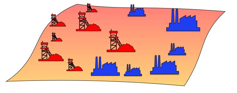
Figure 1. Illustration of Monge optimal transport.

The optimal transport problem is the idea to find a transport plan \(T\) that is a bijection from \(\mathcal{X}\) to \(\mathcal{Y}\), that is to say an assignment so that each mine \(x \in \mathcal{X}\) supplies a unique factory \(y \in \mathcal{Y}\), so that the total transport cost is minimal, where the transport cost \(c(T)\) of a transport plan \(T\) is defined as follows :

\[c(T) = \sum_{x \in \mathcal{X}} c(m, T(m))\]

This is the initial optimal transport problem, illustrated in Figure 1, as formulated by Gaspard Monge in 1781. It has one major mathematical limit and one major philosophical limit (that are in fact related):

• It is not guaranteed that such an optimal transport plan exists
• One might want to relax the constraint that a mine can only provide a unique factory

 

Relaxation of the formulation by Kantorovich

In the 1940s, Leonid Kantorovich proposed the most significant advances since the original problem formulation by encompassing it in a more general framework that has nicer mathematical properties.

Let us define the transport cost matrix \(M_{XY} = [c(x_i,y_i)]_{ij}\). The set of all admissible transport plans, also called couplings, is:

\[U(\mu,\nu) = \{P \in \mathbb{R}_{+}^{m \times n} \vert P1_m=\mu, P^T 1_n = \nu \}\]

This is the same kind of transport plan than in the Monge formulation in the sense that it aims to transport distribution mass \(\mu\) to distribution \(\nu\), except that it gets rid of the uniqueness in the “mine-to-factory” assignment.

Note that the Monge formulation is equivalent to requiring the matrices to be permutation matrices

The cost remains similar except that it is now formulated with matrix :

\[\min_{P \in U(\mu, \nu)} \sum_{i=1, j=1}^{m,n} P(i,j)c(x_i,y_j) = \min_{P \in U(\mu, \nu)} \langle P,M_{XY} \rangle\]

where \(\langle \cdot, \cdot \rangle\) designates the Frobenius distance.

Figure 2. Illustration of Kantorovich optimal transport and cost matrix.

 

Discrete vs continuous

The Monge and Kantorovich formulations of optimal transport have been presented above in the discrete case. One reason for that is that it is well-suited to computer-related problems. However, what is discussed here can be extended to continuous measures and even semi-continuous cases, as illustrated in Figure 3. In the continuous case, the Monge and Kantorovich problems are the following :

\[\text{(M)} \qquad \underset{T_{\# \mu} = \nu}{\inf} \int_X c(x,T(x)) \mathrm{d} \mu(x)\] \[\text{(K)} \qquad \underset{\gamma \in \Gamma(\mu, \nu)}{\inf} \int_X c(x,y) \mathrm{d} \gamma(x,y)\]

where \(T\) is a transport map from \(X\) to \(Y\) and \(\Gamma(\mu, \nu)\) denotes the collection of all probability measures on \(X \times Y\) with marginals \(\mu\) on \(X\) and \(\nu\) on \(Y\) (continuous equivalent of \(U(\mu, \nu)\) above).

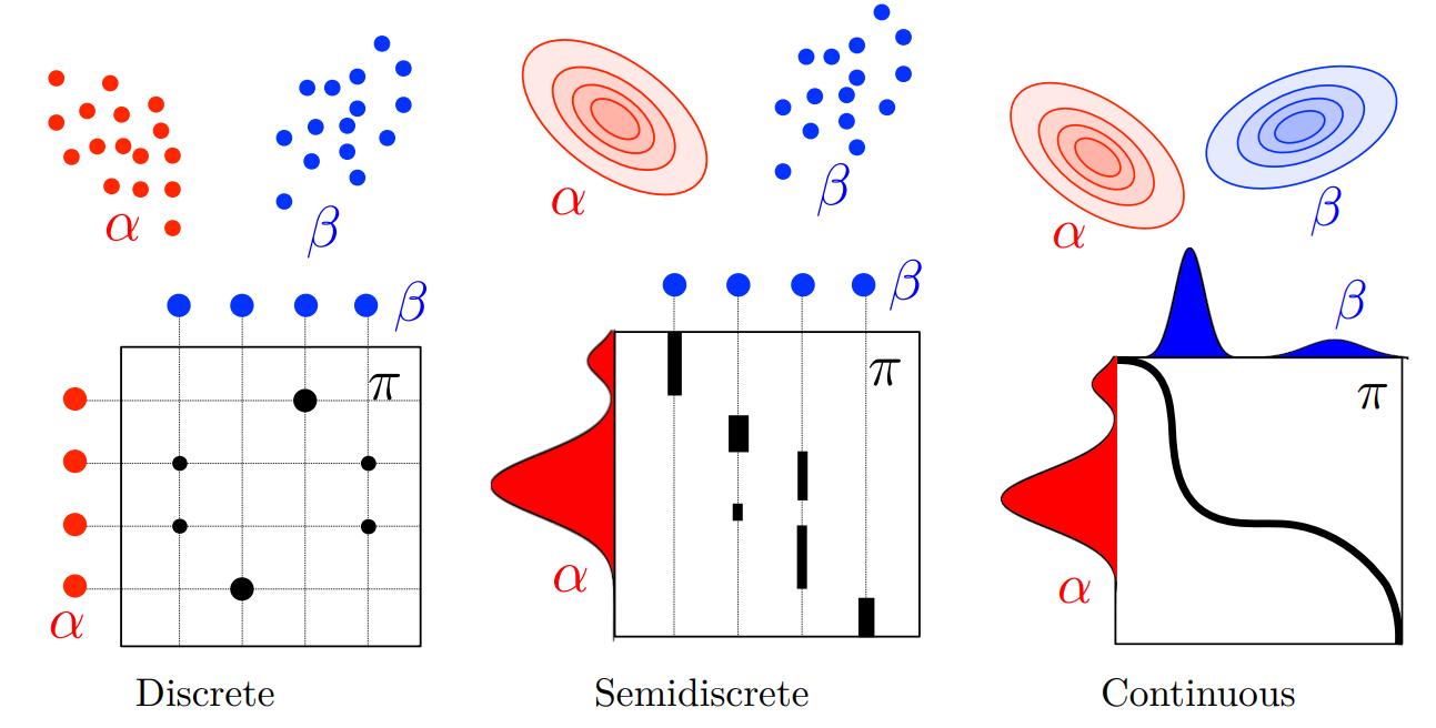
Figure 3. Examples of transort plans in the discrete, semidiscrete and continuous cases.

 

Wasserstein distance and barycenter

For \(p \in [1, +\infty]\) and \(d(\cdot, \cdot)\) a distance, the following quantity defines a distance between two distributions \(\mu\) and \(\nu\) :

\[W_p(\mu, \nu) = (\underset{\gamma \in \Gamma(\mu, \nu)}{\inf} \int_X d^p(x,y) \mathrm{d} \gamma(x,y))^{\frac{1}{p}}\]

Given a set of measures \(\{b_s\}_{s=1,...,S}\), one way to define the barycenter of these measures is :

\[\underset{a}{\min} \sum_{s=1}^{S} \lambda_s W_p^p(a,b_s)\]

where \(\lambda_1,...,\lambda_S\) are the weights given to each distribution.

 

Limits for practical applications

Although properties of existence and uniqueness have been demonstrated for optimal transport for the Kantorovich formulation, as well as equivalence between Monge and Kantorovich’s formulations under certain conditions, there remains several major practical limitations for optimal transport to be directly applied in high dimensionality:

• If the source and target distributions have respectively \(m\) and \(n\) supports points, the solution of optimal transport can be found at best at cost \(O((n+m)nm\log(n+m))\), which is way to expensive for large datasets.
• The optimal transport plan can be “noisy” or “irregular” with respect to inputs.
• The optimal solution \(P^*\) may not be unique and has no meaningful Jacobian with respect to inputs \(X\) or \(Y\), as illustrated in Figure 4.
• The optimal transport plan is bounded to the points that are given when it is computed. One important unanswered question is what happens when a new point is given.
• One may want to compute an optimal transport between distributions that don’t live in the same space or that differ in mass (non equal to 1). Is it possible and how to do it?
• The computation of Wasserstein distance suffers from the curse of dimensionality.

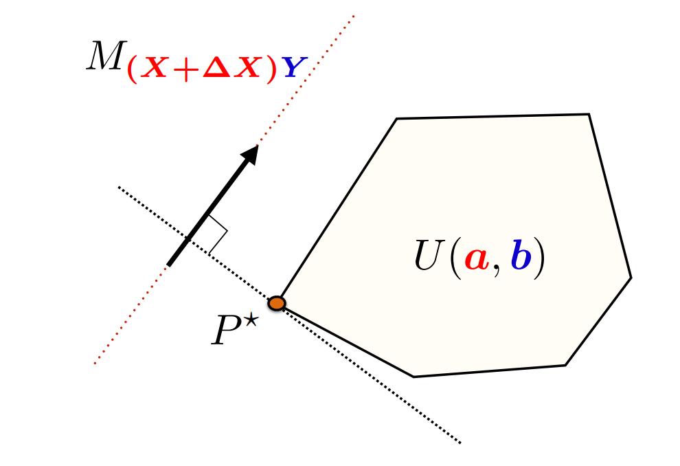
Figure 4. Illustration of a limitation of optimal transport for modern applications.

All these questions are crucial for optimal transport to be applied to large datasets and deep learning. It is because satisfying answers have been found that optimal transport has now been in use for a few years in these domains. The next section aims to present some solutions to the problems listed above.

 

Adaptation of optimal transport to high-dimension problems

Simple 1D case and Sliced Wasserstein distance

In the 1-dimension case with simple distance \(d(x,y) = \vert x - y \vert^p\) with \(p \geq 1\), the optimal tranport plan is trivial when the point \(x_i\) and \(y_i\) are orderer (see Figure 4). Hence, the optimal transport problem is solved in time \(O(n\log n + m \log m)\) (time required to sort the sets of points), which is way more advantageous than the general case.

Figure 5. 1D case for order points. The mass from source points are systematically assigned to target point at leftmost point that is not already filled.

From this property can be derived a strategy “in the philosophy” (in the sense that is does not hold the same properties than real optimal transport) of transport : given points in n-dimension, they are projected to a random direction \(\epsilon \in \mathbb{R}^n\) and the Wasserstein distance is computed on this 1D direction. By repeating this operation (Monte-Carlo method), the n-dimension optimal transport plan is approached.

Recent derivatives of this principle include spherical sliced Wassertein¹ and convolution sliced Wasserstein².

 

Entropy regularization and Sinkhorn algorithm

In 2013, Marco Cuturi introduced a simple method to regularize the classical optimal transport problem and speed up significantly the computation of such transport plan³. It adds to the usual cost to minimize a term of entropy as follows (Regularized Wasserstein distance) :

\[W_\gamma(\mu, \nu) = \underset{P \in U(\mu, \nu)}{\langle P, M_{XY} \rangle} - \gamma E(P)\]

where \(E(P) = - \sum_{i,j} P_{i,j}(\log P_{i,j} - 1)\) and \(\gamma \geq 0\) defines the amount of entropy regularization in the transport plan. This reformulation transforms the problem from a linear programming to a convex problem, which makes its solution way easier to compute. In particular, Sinkhorn algorithm can be leveraged. It states that there exists a unique \(u \in \mathbb{R}_+^n\) and \(v \in \mathbb{R}_+^n\) such that :

\[P_\gamma \overset{def}{=} \underset{P \in U(\mu, \nu)}{\textrm{arg min }} \langle P, M_{XY} \rangle - \gamma E(P) = \textrm{diag}(u)K\textrm{diag}(v) \qquad \textrm{with} \; K\overset{def}{=}\rm e^{-M_{XY}/\gamma}\]

\(u\) and \(v\) can simply be obtained by repeating the two following steps (with random initialization) until convergence :

\[u=a/Kv\] \[v=b/K^T v\]

In most of the derivatives from regularized/alternative optimal transport problems presented after, there exists a way to modify this classical Sinkhorn algorithm to fit the new problem.

The effect of regularization on the optimal transport plan is observable on the Figures 6 and 7 hereunder. The greater the \(\gamma\) is, the more weights of the points are distributed to multiple points. In the limit where \(\gamma\) tends to infinity, we obtain a uniform coupling matrix. On the continuous transport plan, one can observe that a higher entropy leads to a blurrier matrix.

Figure 6. Illustration of the effect of increasing entropy regularization on 1D continuous optimal transport.

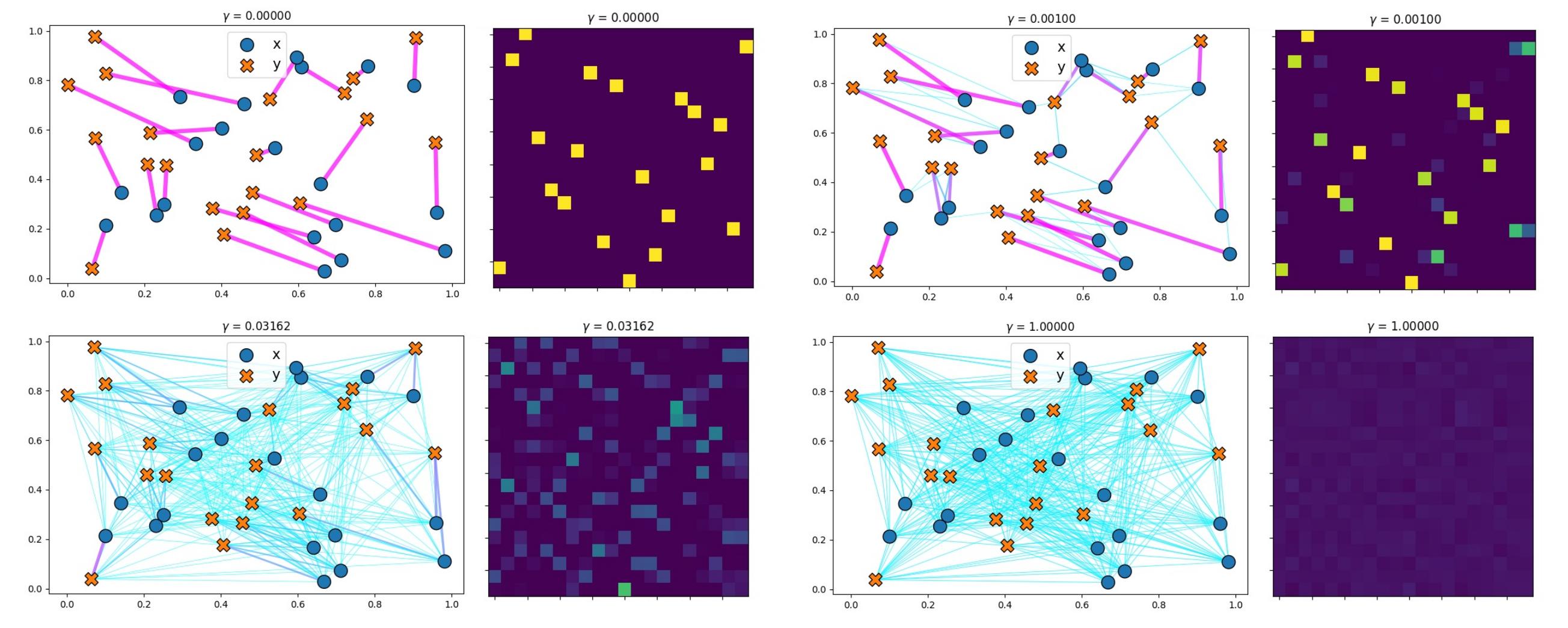
Figure 7. Illustration of the effect of increasing entropy regularization on discrete optimal transport.

 

Low-rank decomposition

Computational efficiency can be further improved by decomposing the coupling matrix into a matrix of (low) rank \(r\) :

\[P = QD(1/g)R^T\]

with \(Q \in U(\mu, g)\), \(R^T \in U(g, \nu)\), \(g\) is a new marginal of size \(r\) and \(D(1/g)\) is a diagonal matrix. This acts like if the transport transited through r virtual anchors points. It is in a sense like doing K-means simultaneously for two measures. The decomposition obviously affects the shape of the coupling matrix, which is now composed of blocks, as illustrated in Figure 8 and 9. There exists a modified Sinkhorn algorithm to handle this low-rank formulation.

Figure 8. Illustration of the effect of the rank (and entropy) on 1D continuous optimal transport.

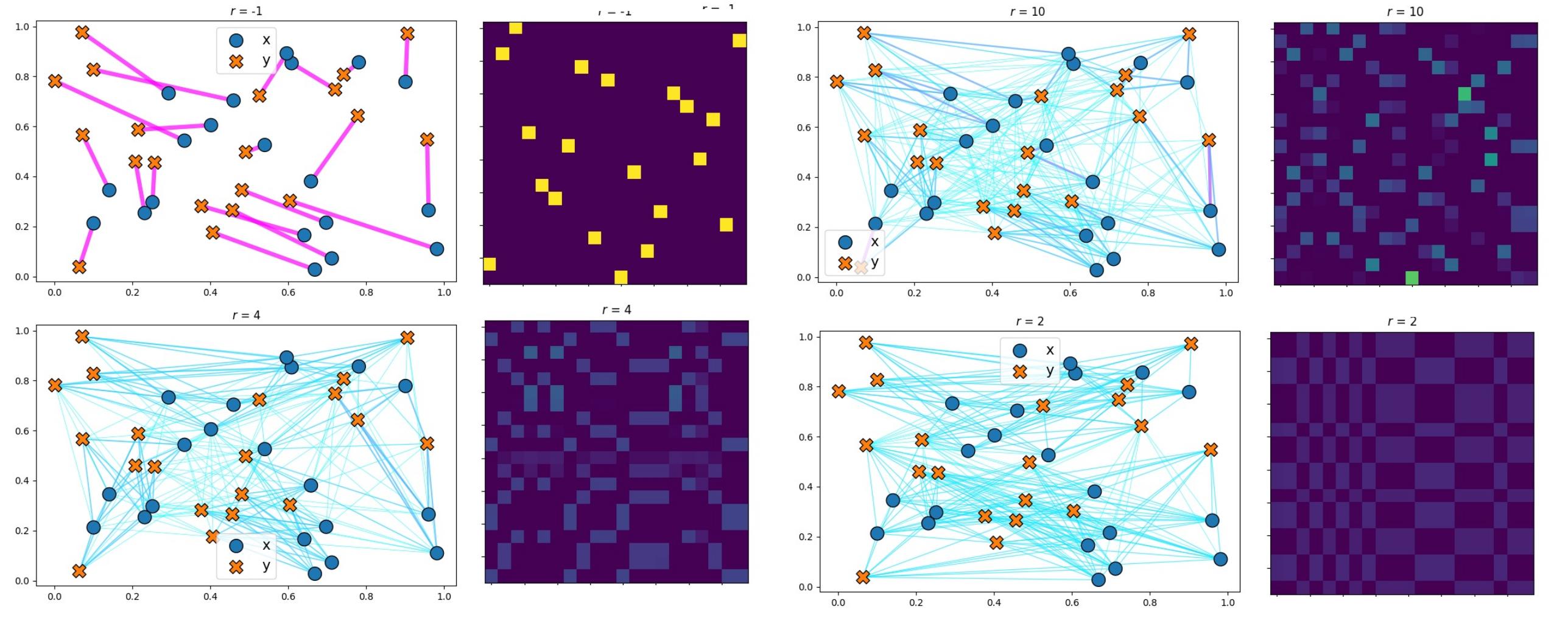
Figure 9. Illustration of the effect of the decomposition of the coupling matrix into a low-rank matrix.

 

“Unstable” assignment and non-differentiability

As problems in classical optimal transport, we mentionned that the optimal transport plan \(P^*\) is not differentiable with respect to \(X\) or \(Y\) and that the assignement from source mass points to target mass points is “noisy” or “unstable”. The first phenomenon is illustrated in Figure 4 hereabove and the second one is illustrated in Figure 8. When points move in space, the optimal transport plan can make “jumps”, that are not desirable for robustness.

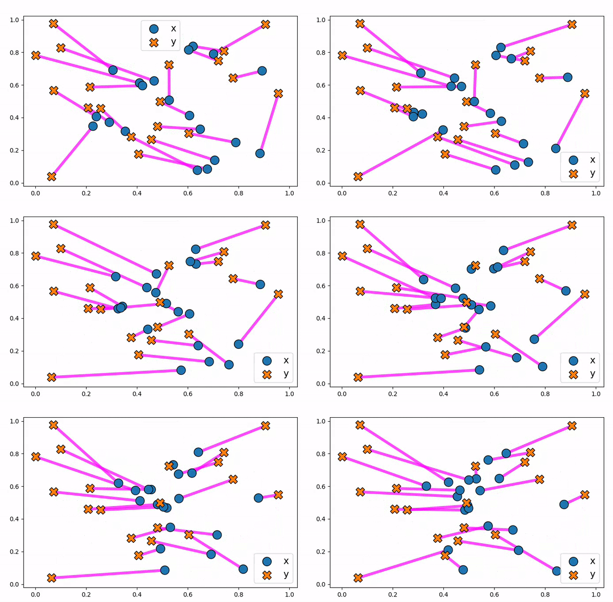
Figure 10. Animation to show how an optimal transport plan can be unstable to small changes in data points.

One way to solve this issue is to move from discrete formulation to continuous transport plan via Monge maps (Figure 11). The optimal transport plan can be parametrized and approximated by neural networks such as Input Convex Neural Networks⁴ or Normalizing Flows⁵.

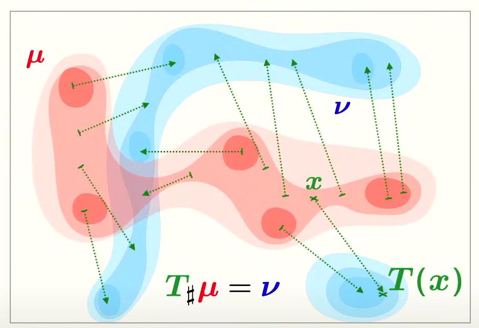
Figure 10. Example of Monge map.

 

(Fused) Gromov-Wasserstein Optimal Transport

The Gromov-Wasserstein Optimal Transport extends the classical optimal transport problem to the case where the source and target points do not live in the same space. In that case, one cannot directly define a cost function to link the points from \(X\) and \(Y\). To solve this, the idea is to build a kind of isometric mapping, where, if both spaces have a cost function, we want to preserve the distance between the points. The problem can be written as follows :

\[P^* ⁼ \underset{P1_m=\mu, P^T 1_n=\nu}{\textrm{arg min }} \sum_{i, i', j, j'} P_{ij}P_{i', j'}(c_1(x_i, x_j) - c_2(y_{i'}, y_{j'})^2)\]

where \(c_1\) and \(c_2\) and cost function respectively defined on \(X\) and \(Y\).

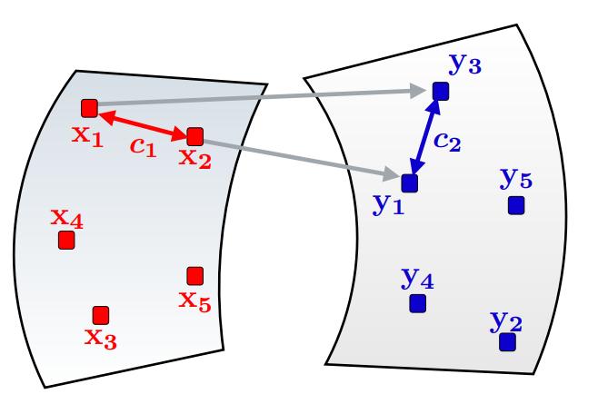
Figure 11. Gromov-Wasserstein Optimal Transport.

In the example shown of Figure 11, if \(x_1\) is assigned to \(y_3\) and \(x_2\) to \(y_1\), we would like \(c_1(x_1, x_2)\) to be equal to \(c2_(y_3, y_1)\).Gromov-Wasserstein optimal transport is compatible with entropy regularization and low-rank formulation.

If each point in \(X\) and \(Y\) is embedded with a feature vector \(f \in \mathbb{R}^b\), this data can be added as an additional term in the minimization problem (associated with a cost function \(c_3\)): \(\alpha \sum_{i,j} P_{i,j}c_3(f(x_i, y_j))\). This is called Fused Gromov-Wassertein Optimal Transport. This formulation can be leveraged in graphs for instance or in dynamic problems.

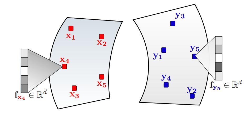
Figure 11. Gromov-Wasserstein Optimal Transport.

Use of optimal transport for deep learning

Now that a lot of concepts of optimal transport have been introduced and that computational tricks have been proposed to adapt the inital optimal transport problem to large datasets, we can present several papers in the deep learning domain in which optimal transport have been directly used.

• The most known one is maybe the Wassertein GAN⁶, where the authors have used Wasserstein distance as a cost function instead of the typical discriminator to stabilize the training of the network, getting rid of problems such as mode collapse and providing meaningful learning curves useful for debugging and hyperparameter searches.

 

• Coupled VAE (C-VAE)⁷ formulates the VAE problem as one of optimal transport between the prior and data distributions. The C-VAE allows greater flexibility in priors and natural resolution of the prior hole problem by enforcing coupling between the prior and the data distribution.

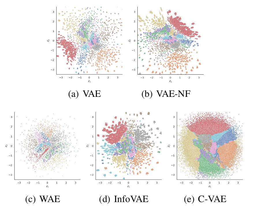
Figure 12. C-VAE. Samples from aggregated posterior. Each color represents a digit

 

• Because of its inherent property to match distributions, one of the most common applications of optimal transport is domain adaptation^{8 9}.

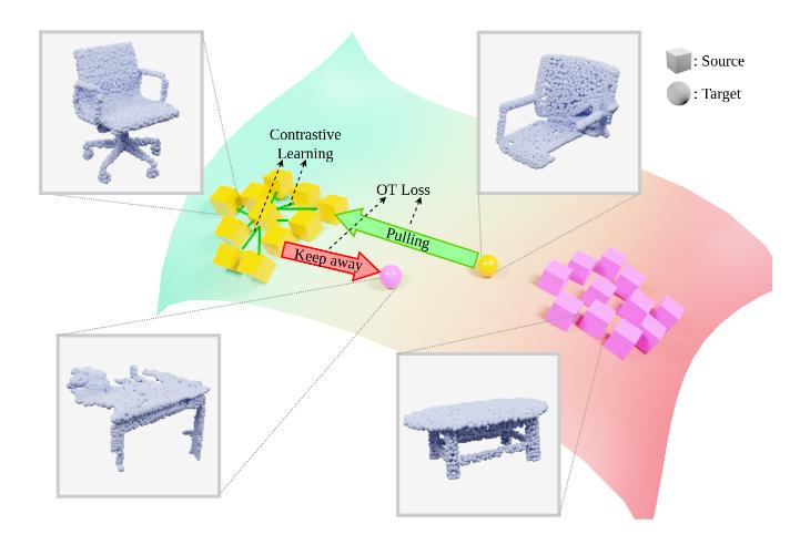
Figure 13. Example of use of optimal transport for domain adaption of point clouds.

 

• It can also be used to improve multimodal representation learning^{10 11 12}.

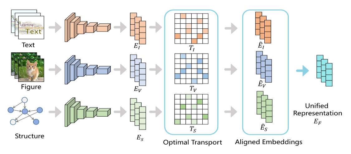
Figure 14. Example of use of optimal transport for heteregeneous multimodal representation learning.

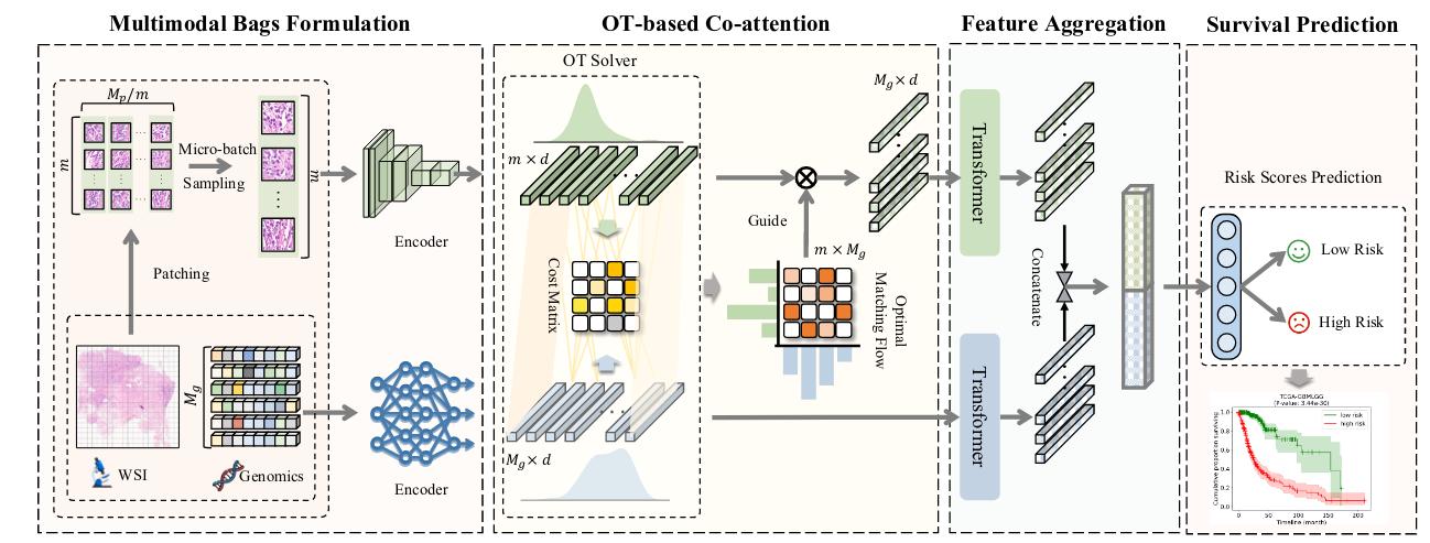
Figure 15. Example of use of optimal transport for multimodal representation learning for whole slice imaging.

 

• Optimal transport has also been applied when prototypes/anchors are useful^{10 13}.

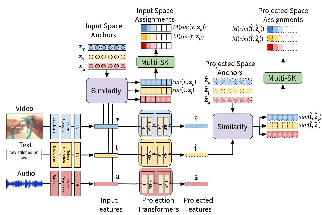
Figure 16. Example of use of optimal transport for anchoring.

 

• It has also been used to improve zero-shot performance of foundation models

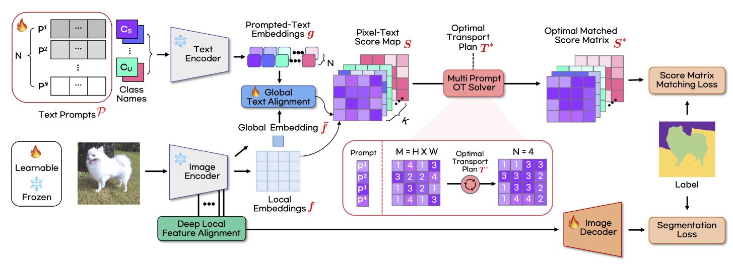
Figure 17. Example of use of optimal transport for zero-shot classification from foundation models.

 

• Optimal transport can also be leveraged to model dynamic and temporal evoluations^{14 15}.

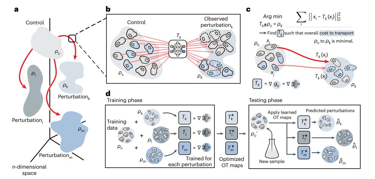
Figure 18. CellOT, a framework for learning the response of individual cells to a given perturbation.

 

Conclusion

Optimal transport is field of mathematics that gained a lot of popularity during the recent decades. The principle is to transport the mass of a source probability distribution to a target probability distribution in a way that minimize the cost of transfer. Although quite impractical to use in computer and data science at first, optimal transport has benefit from breakthoughs that have provided solutions to some of its major limits, in particular the high computational cost. Over the last few years, an increasing number of papers using optimal transport have appeared at the main deep learning conferences, in various sub-domains such as domain adaptation or multimodal representation learning. There are still a lot of remaining topics in optimal transport for data science that has not been discussed in this post, such as unbalanced optimal transport, mini-batch optimal transport, stochastic transport, their link with score-based models,JKO objective, etc.

 

References

1. C. Bonet, P. Berg, N. Courty, F. Septier, L. Drumetz, M.-T. Pham, Spherical Sliced-Wasserstein, ICLR 2023. ↩

2. K. Nguyen, N. Ho, Revisiting Sliced Wasserstein on Images: From Vectorization to Convolution, NeurIPS 2022. ↩

3. M. Cuturi, Sinkhorn Distances: Lightspeed Computation of Optimal Transport, NeurIPS 2013. ↩

4. B. Amos, L. Xu, J. Z. Kolter, Input Convex Neural Networks, PMLR 2017. ↩

5. F. Coeurdoux, N. Dobigeon, P. Chainais, Learning Optimal Transport Between two Empirical Distributions with Normalizing Flows, Machine Learning and Knowledge Discovery in Databases. ECML PKDD 2022. ↩

6. M. Arjovsky, S. Chintala, L. Bottou, Wasserstein Generative Adversarial Networks, PMLR 2017. ↩

7. X. Hao, P. Shafto, Coupled Variational Autoencoder, PMLR 2023. ↩

8. N. Courty, R. Flamary, D. Tuia, A. Rakotomamonjy, Optimal Transport for Domain Adaptation, IEEE Transactions on Pattern Analysis and Machine Intelligence, 2017. ↩

9. S. Katageri, Arkadipta De, C. Devagupt, VSSV Prasad, C. Sharma, M. Kaul, Synergizing Contrastive Learning and Optimal Transport for 3D Point Cloud Domain Adaptation, WACV 2024. ↩

10. S. Swetha, M. Nayeem Rizve, N. Shvetsova, H. Kuehne, Mubarak Shah, Preserving Modality Structure Improves Multi-Modal Learning, ICCV 2023. ↩ ↩²

11. Z. Cao, Q. Xu, Z. Yang, Y. He, X. Cao, Q. Huang, OTKGE: Multi-modal Knowledge Graph Embeddings via Optimal Transport, NeurIPS 2022. ↩

12. Y. Xu, H. Chen, Multimodal Optimal Transport-based Co-Attention Transformer with Global Structure Consistency for Survival Prediction, ICCV 2023. ↩

13. M. Caron, I. Misra, J. Mairal, P. Goyal, P. Bojanowski, A. Joulin, Unsupervised Learning of Visual Features by Contrasting Cluster Assignments, NeurIPS 2024. ↩

14. C. Bunne, S. G. Stark, G. Gut, J. Sarabia Del Castillo, M. Levesque, K.-V. Lehmann, L. Pelkmans, A. Krause, G. Rätsch, Learning single-cell perturbation responses using neural optimal transport, Nature Methods, 2023. ↩

15. M. Masias, M. A. González, G. Piella, Predicting structural brain trajectories with discrete optimal transport normalizing flows, Poster in Workshop: Medical Imaging meets NeurIPS 2022. ↩