Introduction to Graph Neural Networks

Additional References

• This Distill paper¹ published by Sanchez-Lengeling et al. in 2021 is another good introduction to GNNs in a more general context, with lots of (interactive) examples.
• Model architectures presented are not exhaustive and were chosen for their popularity and relevance in the field. A comprehensive review², published by Zhou et al. in 2020, provides a taxonomy of many more GNN methods and their applications.
• The benchmark study by Dwivedi et al.³ in 2022 provides detailed insights into GNN design that are too advanced for this introductory tutorial, such as edge features and positional encodings.

 

Summary

• Introduction
  • What is a graph and why use it?
  • Formal representation
• GNN task types
  • Graph-level vs Node-level vs Edge-level tasks
  • Focus on graph-level classification
• Graph Deep Learning paradigm
  • Message passing intuition
  • Mathematical formalism
• Encoder architectures
  • GCN • Graph Convolutional Network
  • GAT • Graph Attention Network
  • GIN • Graph Isomorphism Network
• References

 

Introduction

What is a graph and why use it?

Imagine an image: a structured grid of pixels where each pixel’s color or intensity doesn’t exist in isolation but is influenced by those immediately around it. Now, consider a graph: instead of a fixed grid, you have a collection of nodes, each carrying its own information, interconnected by edges that define their relationships.

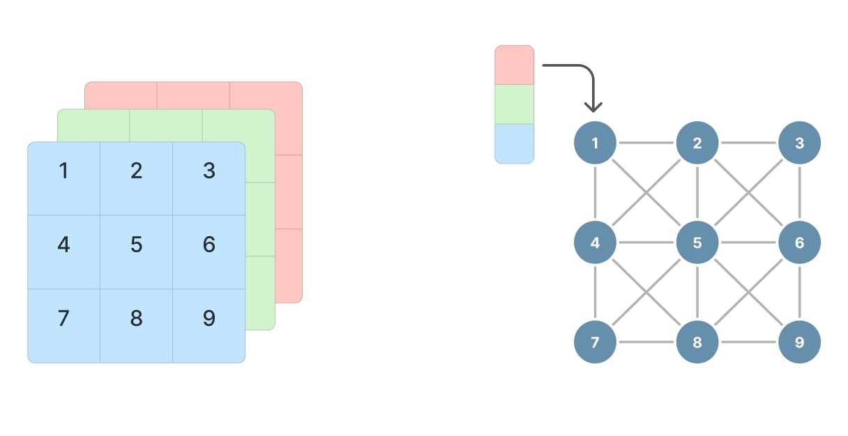
Figure 1. Image and graph representation.

 

The graph abstraction is particularly powerful for representing data where interactions and relationships are non-Euclidean and irregular. Unlike the Euclidean grid-like structure of images, graphs can capture arbitrary patterns of connectivity, making them ideal for modeling social networks, transportation systems, molecular structures, and more.

 

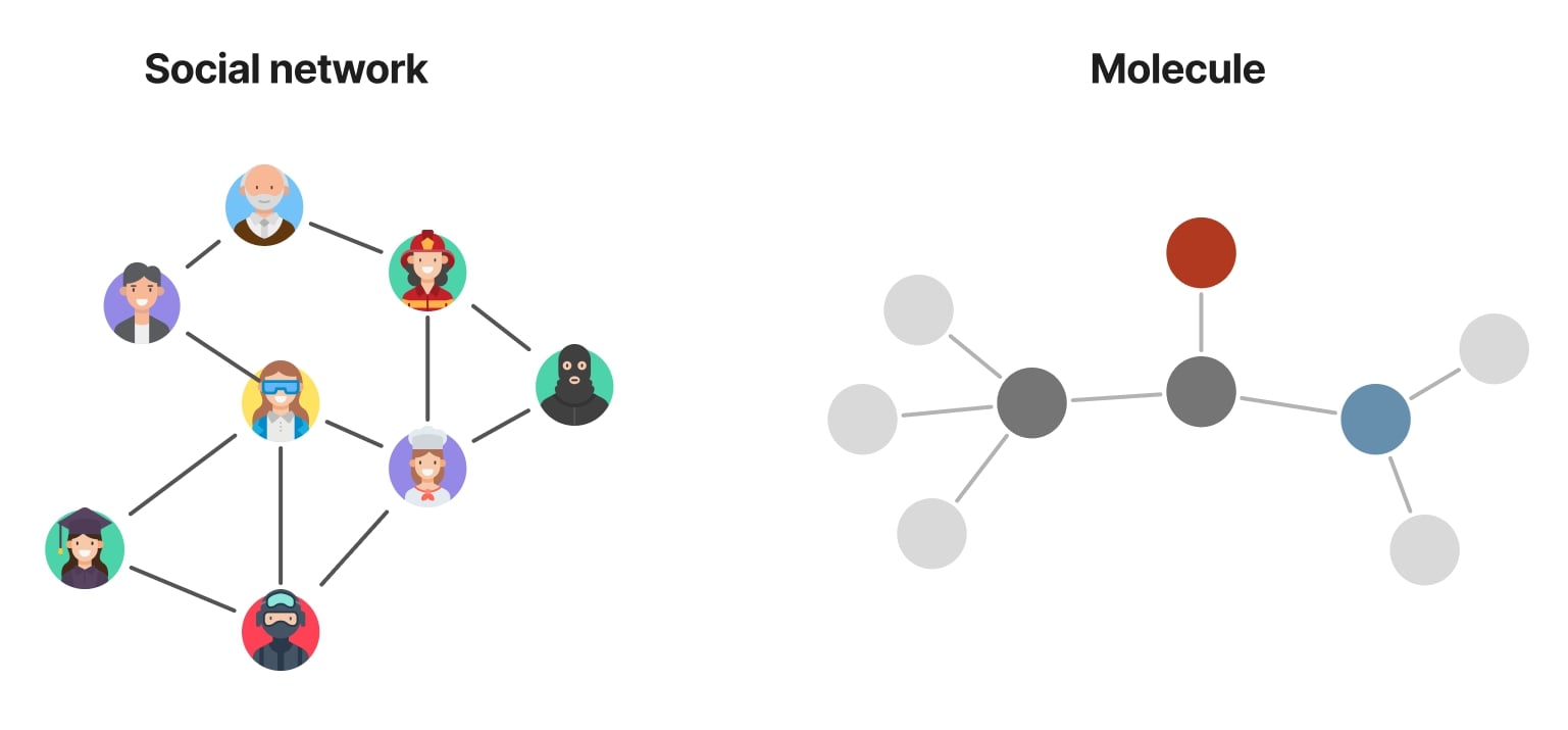
Figure 2. Example of graph applications.

 

Whereas a pixel in an image is defined in space by its own coordinates, a node in a graph has no coordinates. Rather, it is defined in space only in relation to its neighbors. Think of it as an image where the “neighboring” pixels aren’t just those directly adjacent, but can be any pixels that share a meaningful connection, forming a network that captures more complex and abstract interactions.

 

Formal representation

Graph definition

A graph is formally defined as \(G = (V, E)\), where:

• \(V\) is a set of nodes (or vertices)
• \(E \subseteq V \times V\) is a set of edges (or links)

Note: More general definitions also include \(U\) to represent global attributes (or a master node)^{2 1}.

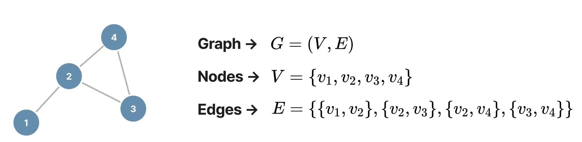
Figure 3. Undirected graph.

 

In the case of directed graphs, each edge is an ordered pair \((v_i, v_j)\), where \(v_i\) is the source node and \(v_j\) is the target node. This contrast with undirected graphs, where an edge is an unordered pair \((v_i, v_j) = (v_j, v_i)\) as presented in Figure 3.

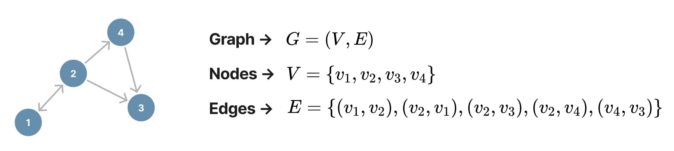
Figure 4. Directed graph.

 

Adjacency matrix

One common representation of a graph \(G\) is through its adjacency matrix \(A \in \mathbb{R}^{N \times N}\), where \(N = |V|\), i.e. the number of nodes. The adjacency matrix is a binary matrix that encodes the presence of edges between nodes such as:

\[A_{ij} = \begin{cases} 1 & \text{if } (v_i, v_j) \in E, \\ 0 & \text{otherwise}. \end{cases}\]

 

In the case where \(G\) is undirected, the adjacency matrix is symmetric: \(A = A^T\):

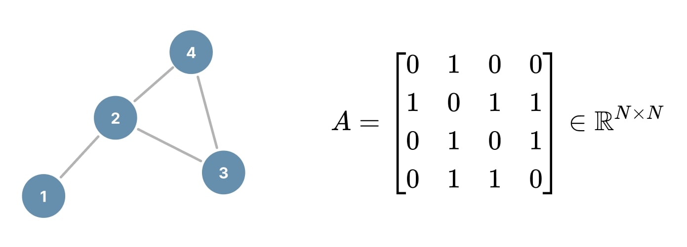
Figure 5. Adjacency matrix example.

 

Node and edge features

The features of a node are denoted by \(x_i \in \mathbb{R}^{d_n}\), where \(d_n\) is the number of features per node. Similarly, the features of an edge \((v_i, v_j)\) (directed or not) are denoted by \(e_{ij} \in \mathbb{R}^{d_e}\), where \(d_e\) is the number of features per edge.

 

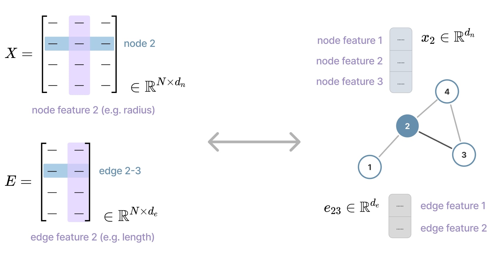
Figure 6. Node and edge features matrix.

 

In typical GNNs, node features will be aggregated and updated across neighbors along the model’s layers. Thus, node features at layer are usually denoted as \(l\) is \(h_i^{(l)} \in \mathbb{R}^{d_n^{(l)}}\), where \(d_n^{(l)}\) is the number of features per node at layer \(l\). As for the edge features, they are typically not updated through layers, so their notation is generally unchanged: \(e_{ij}^{(l)} \in \mathbb{R}^{d_e^{(l)}}\). Thus, a general matrix notation is:

 

\[H^{(l)} = \begin{bmatrix} h_1^{(l)} \\ h_2^{(l)} \\ \vdots \\ h_N^{(l)} \end{bmatrix} \in \mathbb{R}^{N \times d_n^{(l)}} \quad \text{with} \quad X = H^{(0)}\] \[E^{(l)} = \begin{bmatrix} e_{12}^{(l)} \\ e_{23}^{(l)} \\ \vdots \\ e_{N-1,N}^{(l)} \end{bmatrix} \in \mathbb{R}^{N \times d_e^{(l)}} \quad \text{with} \quad E = E^{(0)}\]

 

As is common in other machine learning domains, we denote respectively \(Y\) and \(\hat{Y}\) the prediction target and the predicted output.

 

GNN task types

Graph-level vs Node-level vs Edge-level tasks

In graph learning, tasks are generally categorized based on the level at which predictions are made. Three main categories are typically considered²:

 

Node-level tasks

Here, the goal is to predict a label or value for each individual node, based on both the node’s intrinsic features and the information aggregated from its neighbors. The prediction for each node \(\hat{y_i}\) can be formulated as:

\[\hat{y_i} = f_{\text{node}}(h_i^{(L)})\]

Examples:

• Social network: Classifying users (for instance, determining whether a user is influential).
• Community detection: Identifying clusters or communities of nodes with similar characteristics.

Methods:

• Multi-layer message passing to refine local node representations by incorporating contextual information from their neighborhoods.

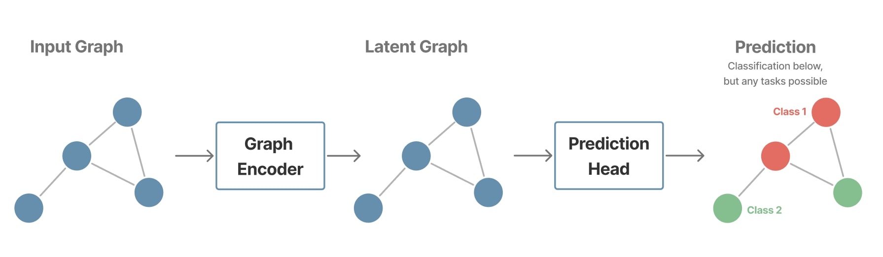
Figure 8. Example of a node-level pipeline.

 

Edge-level tasks

These tasks focus on the interactions between nodes and aim to predict the presence or nature of a connection between two nodes. This often involves constructing an edge representation from the features of the connected nodes. The prediction for each edge \(\hat{y_{ij}}\) can be formulated as:

\[\hat{y_{ij}} = f_{\text{edge}}(h_i^{(L)}, h_j^{(L)}, e_{ij}^{(L)})\]

Examples:

• Link prediction: Determining whether a connection exists between two nodes, which is useful in recommendation systems or for discovering new relationships in social networks.
• Edge classification: Identifying the type or strength of the relationship between two nodes in multi-relational graphs.

Methods:

• Creating edge representations through operations such as concatenation, absolute difference, or other combinatorial methods applied to the node features.
• Using scoring functions to estimate the likelihood or strength of the connection between nodes.

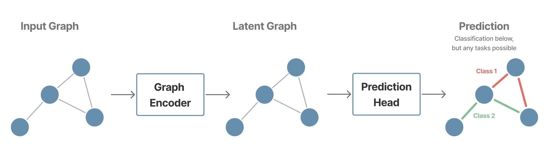
Figure 9. Example of an edge-level pipeline.

 

Graph-level tasks

These tasks involve predicting a property or label for the entire graph. To do this, node representations are typically aggregated using a global pooling operation to produce an overall graph representation. The graph prediction \(\hat{y_G}\) can be formulated as:

\[h_G = \text{readout}(H^{(L)}) \\ \hat{y_G} = f_{\text{graph}}(h_G)\]

Examples:

• Computational chemistry: Predicting molecular properties (e.g., chemical activity) based on the molecular graph structure.
• Social network analysis: Classifying an entire network to identify its type or activity level.

Methods:

• Multi-layer message passing to refine local node representations by incorporating contextual information from their neighborhoods.
• Readout step that transforms local node representations into a comprehensive global graph representation.

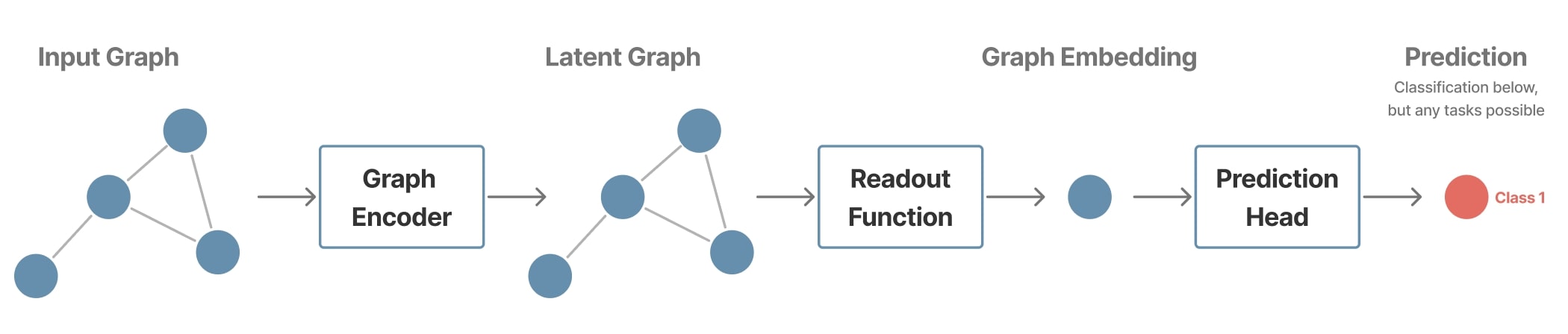
Figure 7. Example of a graph-level pipeline.

 

Focus on graph-level classification

In graph-level classification tasks, the objective is to predict a label for the entire graph \(G\). This requires combining the information contained in all node embeddings into a single vector representation \(h_G\) via a readout function. This graph embedding can then be used to make predictions about the graph as a whole.

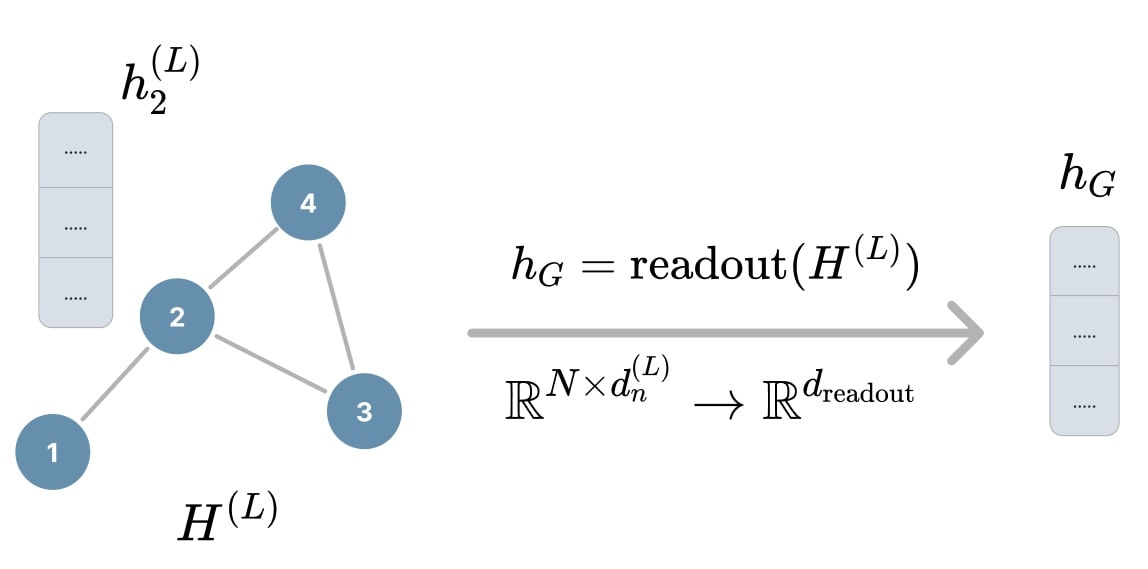
Figure 10. Readout for graph pooling.

 

The figure above illustrates this principle:

• After \(L\) layers of message passing, each node \(v_i\) has an embedding \(h_i^{(L)}\).
• All node embeddings are stacked into a matrix \(H^{(L)} \in \mathbb{R}^{N \times d_n^{(L)}}\), where \(N\) is the number of nodes and \(d_n^{(L)}\) is the node embedding size.
• A \(\text{readout}\) function is then applied to this matrix to obtain a fixed-size graph embedding \(h_G \in \mathbb{R}^{d_{\text{readout}}}\), independent of the number of nodes.

 

Common readout functions

Several readout mechanisms are used in practice. This readout step is essential for enabling GNNs to perform downstream tasks such as graph classification, regression, or retrieval. The choice of readout impacts both expressiveness and model performance, and should be guided by the nature of the graph data and the task. Below are some common readout functions:

Sum pooling: Captures the total signal in the graph; sensitive to graph size.

\[\,\\ h_G = \sum_{v_i \in V} h_i^{(L)} \\ \mathbb{R}^{d_n^{(L)}} \leftarrow \mathbb{R}^{N \times d_n^{(L)}} \\\]

Mean pooling: Normalizes the sum and makes the representation invariant to the number of nodes.

\[\,\\ h_G = \frac{1}{N} \sum_{v_i \in V} h_i^{(L)} \\ \mathbb{R}^{d_n^{(L)}} \leftarrow \mathbb{R}^{N \times d_n^{(L)}} \\\]

Max pooling: Highlights the most prominent features across the graph.

\[\,\\ h_G = \max_{v_i \in V} h_i^{(L)} \quad \text{(element-wise)} \\ \mathbb{R}^{d_n^{(L)}} \leftarrow \mathbb{R}^{N \times d_n^{(L)}} \\\]

More complex readout methods have also been studied, like SortPool⁴ (learn a score per node, rank and select the top k embeddings, then concatenate into a fixed-size graph vector) and GraphTrans⁵ (permutation-invariant Transformer with a global token for self-attention over node embeddings)

 

Classification head

After obtaining the final graph embedding \(h_G\) through a chosen readout function, the next step is to perform classification. As shown in the figure below, we classically use a multi-layer perceptron (MLP) to transform the embedding \(h_G \in \mathbb{R}^{d_{\text{readout}}}\) into a logit vector, which is then converted into a probability distribution over the target classes.

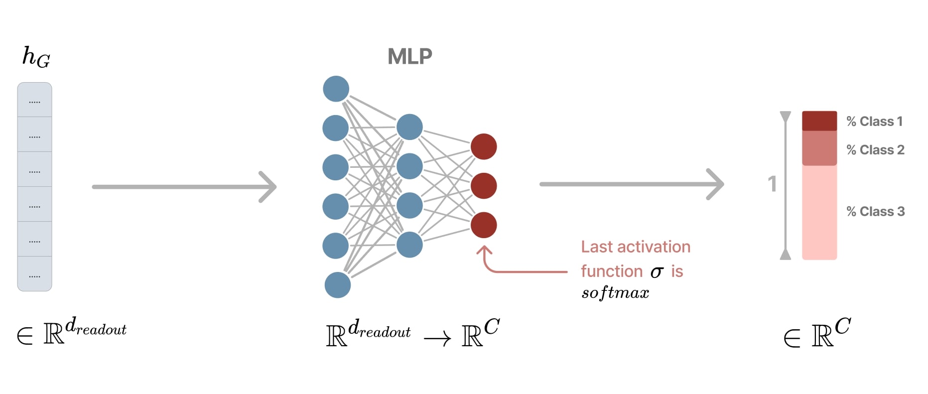
Figure 11. Classification head.

 

Note: While \(h_G\) is used here for graph-level classification, this principle can be extended to other tasks.

• Node-level classification: Instead of a single graph embedding, each node \(v_i\) has an embedding \(h_i\). Each node embedding is passed individually into the same MLP head to obtain per-node class predictions.
• Edge-level classification: Each edge \((v_i, v_j)\) has an embedding \(e_{ij}\). An MLP head can similarly classify each edge by mapping \(e_{ij}\) to a probability distribution over edge classes.

 

Graph Deep Learning paradigm

Message passing^{6 7} is a building block of many popular GNN architectures. Like convolutions for deep vision models, it is a general framework to process and extract features from the data. Typical graph encoders are designed by stacking multiple message passing steps one after the other, to refine features representation on each node (and sometimes edge) in the graph.

Message passing intuition

Every node \(i\) sends a message to each of its neighbors \(j\) and, in turn, receives messages from those neighbors. This mechanism enables local information to be disseminated throughout the graph, allowing each node to incorporate contextual information from its surroundings. The aggregation process has to ensure permutation invariance, since the ordering of neighboring nodes is arbitrary.

 

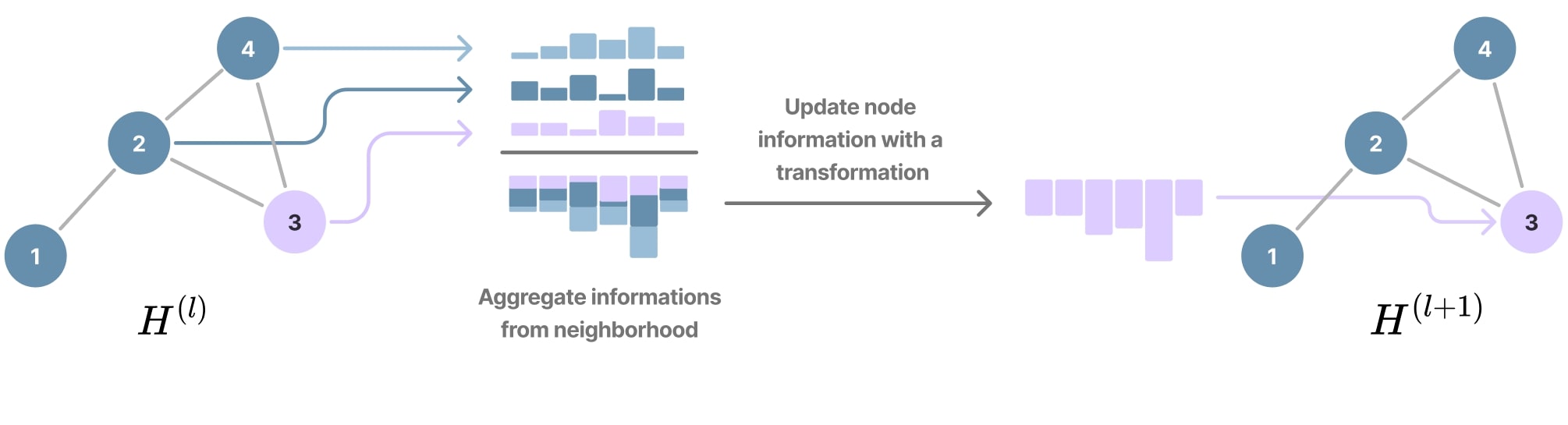
Figure 12. Simple example of message passing (inspired by a figure from Sanchez-Lengeling et al.[^4]).

 

Mathematical formalism

In each layer, every node \(v_i\) updates its feature representation by aggregating messages from its neighbors such as:

\[\,\\ h_i^{(l+1)} = \text{UPDATE}\Bigl( h_i^{(l)}, \; \text{AGGREGATE}\Bigl( \bigl\{ \text{MESSAGE}\bigl( h_j^{(l)}, \, h_i^{(l)}, \, e_{ij}^{(l)} \bigr) \mid j \in \mathcal{N}_i \bigr\} \Bigr) \Bigr) \\\]

With the guarantee that the message passing mechanism is permutation invariant, i.e. the order of messages does not matter. This means that the aggregation function must satisfy the following property to faithfully reflect the graph structure:

\[\,\\ \text{AGGREGATE}\left( \{a, b, c\} \right) = \text{AGGREGATE}\left( \{b, c, a\} \right) = \dots \\\]

Where:

• \(\text{MESSAGE}\): Computes a message from a neighbor \(v_j\) by combining its features \(h_j^{(l)}\) (and optionally the central node’s features \(h_i^{(l)}\) and edge features \(e_{ij}^{(l)}\)).
• \(\text{AGGREGATE}\): A function (e.g., sum, mean, or max) that consolidates messages from all neighbors.
• \(\text{UPDATE}\): Merges the aggregated message with the current node state to produce the updated representation.
• \(\mathcal{N}_i \subset \mathbb{R}\) denote the set of neighbors of \(v_i\).

Note: \(\mathcal{N}_i\) can sometimes includes \(i\) itself, but it is not the convention used in this tutorial.

 

Encoder architectures

In a GNN, the graph encoder plays the main role of transforming input features, such as node and edge attributes, into latent representations that can be used for prediction tasks. The sections below introduce three of the most used architectures which fall under the message passing mechanism.

 

GCN • Graph Convolutional Network

The GCN architecture⁸ is directly inspired by Convolutional Neural Networks (CNNs) and utilizes the adjacency matrix to perform the message passing mechanism through matrix computations. This approach allows for the generalization of convolution operations to graph-structured data, enabling the application of deep learning techniques to non-Euclidean domains⁹.

Normalized augmented adjacency matrix

The problem with the adjacency matrix \(A\), as defined previously, is that only the links of its neighbors are contained. So firstly, to include each node in its own aggregation process, we augment \(A\) with the identity matrix \(Id_N\) to add self-connections (\(A_{ii} = 1\)):

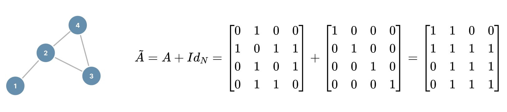
Figure 13. Augmented adjacency matrix.

 

Next we compute the augmented degree matrix \(\tilde{D}\), which represents the number of neighbors for each node (itself included in our case):

\[\tilde{D}_{ii} = \sum_{j=1}^{N} \tilde{A}_{ij} \;\; \Rightarrow \;\; \tilde{D}=\begin{bmatrix} \tilde{d_1}&0&0&0\\ 0&\tilde{d_2}&0&0\\ 0&0&\tilde{d_3}&0\\ 0&0&0&\tilde{d_4} \end{bmatrix} =\begin{bmatrix} 2&0&0&0\\ 0&4&0&0\\ 0&0&3&0\\ 0&0&0&3 \end{bmatrix} \\\]

Finally, the normalized adjacency matrix \(\hat{A}\) is computed using \(\tilde{D}\) based on the spectral graph theory¹⁰. This transformation allows balancing the influence of nodes with varying degrees, since their range of values could might not be normalized w.r.t. their degree, e.g. when using a sum aggregation function. In addition, the normalization helps to stabilize the training process and, especially, to avoid vanishing or exploding gradients.

\[\,\\ \hat{A} = \tilde{D}^{-\frac{1}{2}} \tilde{A} \tilde{D}^{-\frac{1}{2}} = \begin{bmatrix} 0.5 & 0.35 & 0 & 0\\ 0.35 & 0.25 & 0.29 & 0.29\\ 0 & 0.29 & 0.33 & 0.33\\ 0 & 0.29 & 0.33 & 0.33 \end{bmatrix}\]

 

Graph convolutional layer

The convolutional message passing, aggregating and updating steps are performed by the following matrix computation in a GCN layer:

\[H^{(l)} = \sigma \left( \hat{A} \, H^{(l-1)} \, W^{(l)} \right) \;\]

Where:

• \(H^{(l)} \in \mathbb{R}^{N \times d_n^{(l)}}\) is the node features matrix at layer \(l\).
• \(W^{(l)} \in \mathbb{R}^{d_n^{(l-1)} \times d_n^{(l)}}\) is the learnable linear transformation for nodes features.
• \(\sigma\) is a non-linear function such as \(\text{ReLU}\) or \(\text{LeakyReLU}\).

The above formalism remains pretty simple, but below is the detailed computation for one layer of a GCN (the non-linear function \(\sigma\) is omitted for clarity):

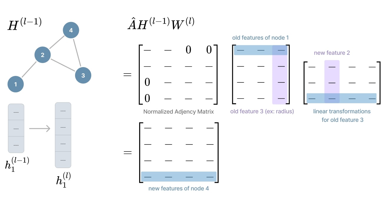
Figure 14. GCN layer details.

 

The above matrix formula can be rewritten in a more explicit form at the node level:

\[\,\\ h_i^{(l)} = \sigma\left( \sum_{j \in \mathcal{N}_i \cup \{ i \}} \frac{1}{\sqrt{\tilde{d_i}} \sqrt{\tilde{d_j}}} \, W^{(l)} \, h_j^{(l-1)} \right)\]

Where:

• \(h_i^{(l)} \in \mathbb{R}^{d_n^{(l)}}\) is the node features at layer \(l\).
• \(W^{(l)} \in \mathbb{R}^{d_n^{(l)} \times d_n^{(l-1)}}\) is the learnable linear transformation.
• \(\tilde{d_i} \in \mathbb{N}\) is the augmented degree of node \(v_i\).
• \(\mathcal{N}_i \subset \mathbb{R}\) denote the set of neighbors of \(v_i\).

 

GAT • Graph Attention Network

The GAT architecture¹¹ popularized a formulation of self-attention for GNNs, inspired by the success of Transformers¹² in NLP that highlighted the importance of dynamically pondering each token in a sequence. Here, the same principle is applied to nodes in a graph, where the attention mechanism allows to weight the influence of each neighbor in the aggregation process.

Self-attention mechanism

Firstly, we compute the attention scores \(a_{ij}\) for all pairs of nodes \((v_i, v_j)\) where \(v_j\) is in the neighborhood of \(v_i\):

\[a_{ij}^{(l)} = \text{LeakyReLU}\left( \mathbf{a}^{(l)^T} \cdot \left[ W^{(l)} h_i^{(l-1)} \parallel W^{(l)} h_j^{(l-1)} \right] \right)\]

Where:

• \(a_{ij}^{(l)} \in \mathbb{R}\) is the attention score between nodes \((v_i, v_j)\).
• \(\mathbf{a}^{(l)} \in \mathbb{R}^{2 \cdot d_n^{(l)}}\) is a learnable attention vector.
• \(W^{(l)} \in \mathbb{R}^{d_n^{(l)} \times d_n^{(l-1)}}\) is a learnable linear transformation.
• \(\parallel\) denotes the concatenation operator.

 

We use the same linear transformation \(W^{(l)}\) for both nodes to project their features into a shared latent space. Their features are then concatenated and multiplied with a 1D vector \(\mathbf{a}^{(l)}\) to compute the attention score. Next, the \(\text{LeakyReLU}\) activation function is applied to introduce non-linearity.

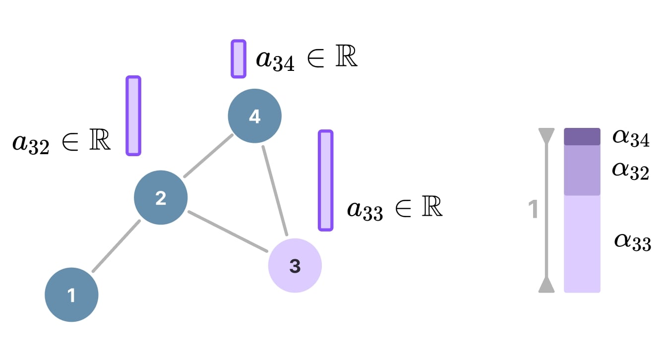
Figure 15. Attention scores and coefficients.

 

But the attention scores (\(a_{ij} \in \mathbb{R}\)) are not normalized yet. As illustrated above, we apply the \(\text{softmax}\) function to obtain the final attention distribution for the neighborhood of a specific node (itself included):

\[\alpha_{ij} = \text{softmax}_j(a_{ij}) = \frac{\exp(a_{ij})}{\sum_{k \in \mathcal{N}_i \cup \{i\}} \exp(a_{ik})}\]

Where:

• \(\alpha_{ij} \in [0, 1]\) is the attention coefficient between nodes \((v_i, v_j)\).
• \(a_{ij}^{(l)} \in \mathbb{R}\) is the attention score between nodes \((v_i, v_j)\).
• \(\mathcal{N}_i \subset \mathbb{R}\) denote the set of neighbors of \(v_i\).

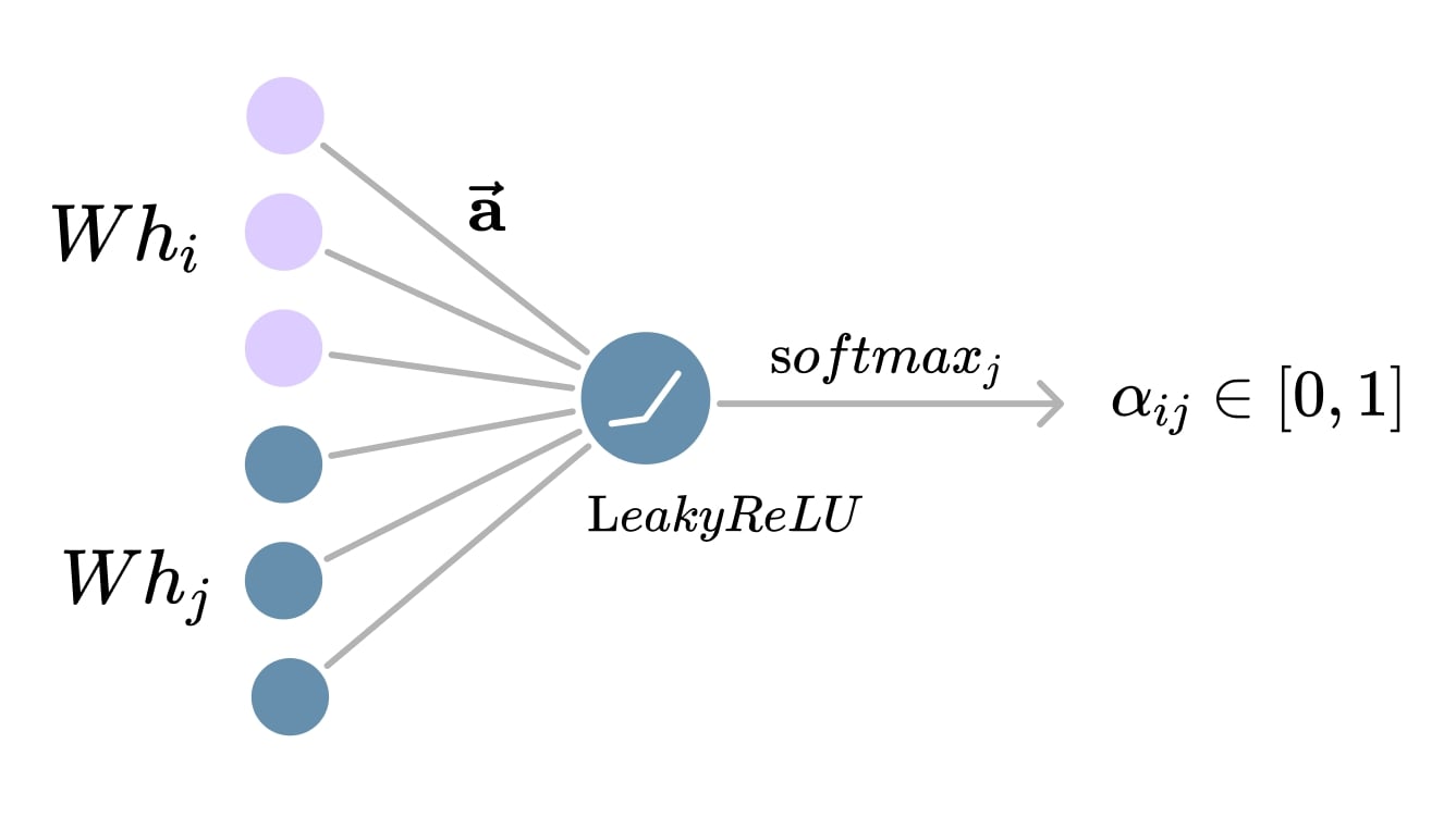
Figure 16. Self-attention computation.

 

Attention aggregation

The final node embedding is computed by aggregating the features that are re-projected by \(W^{(l)}\) in the latent space in which the attention coefficients were computed. The process is really similar to the GCN layer, but with the attention mechanism replacing the degree normalization:

\[\,\\ h_i^{(l)} = \sigma \left( \sum_{j \in \mathcal{N}_i \cup \{i\}} \alpha_{ij}^{(l)} \, W^{(l)} h_j^{(l-1)} \right)\]

Where:

• \(h_i^{(l)} \in \mathbb{R}^{d_n^{(l)}}\) is the node features at layer \(l\).
• \(\alpha_{ij}^{(l)} \in [0, 1]\) is the attention coefficient between nodes \((v_i, v_j)\).
• \(W^{(l)} \in \mathbb{R}^{d_n^{(l)} \times d_n^{(l-1)}}\) is the learnable linear transformation.

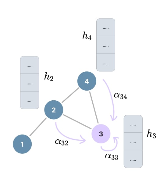
Figure 17. Attention aggregation and update.

 

Multi-head attention aggregation

The attention aggregation process can be further enhanced by using multiple attention heads, each with its own learnable parameters identified by the superscript \(k\) that denote the head id and \(K\) the number of heads. Finally, the outputs of each head are concatenated to produce the final node embedding:

\[\,\\ h_i^{(l)} = \Big\Vert_{k=1}^{K} \sigma \left( \sum_{j \in \mathcal{N}_i \cup \{i\}} \alpha_{ij}^{(l, k)} W^{(l, k)} h_j^{(l-1)} \right)\]

 

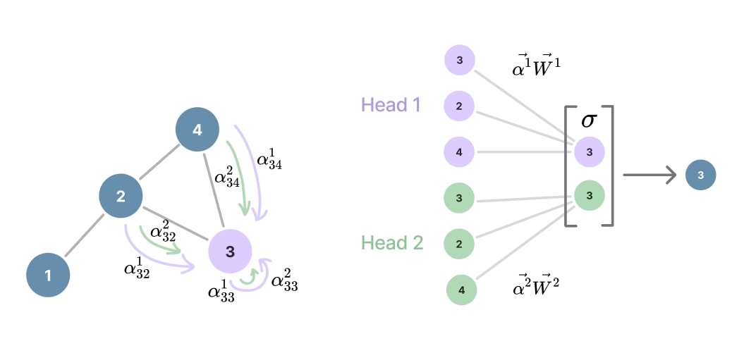
Figure 18. Multi-head attention aggregation and update.

 

GATv2 improvements

The main problem in the standard GAT attention formulation is that the learnable parameters \(W^{(l)}\) and \(\mathbf{a}^{(l)}\) are applied consecutively, and thus can be collapsed into a single linear transformation layer. So the GATv2 architecture¹³ proposes to apply the attention vector \(\mathbf{a}^{(l)}\) after the \(\text{LeakyReLU}\) function:

\[\,\\ \text{GAT (2018):} \;\;\;\; a_{ij}^{(l)} = \text{LeakyReLU}\left( \mathbf{a}^{(l)^T} \cdot \left[ W^{(l)} h_i^{(l-1)} \parallel W^{(l)} h_j^{(l-1)} \right] \right) \\ \text{GATv2 (2021):} \;\;\;\; a_{ij}^{(l)} = \mathbf{a}^{(l)^T} \cdot \text{LeakyReLU} \left( W^{(l)} \left[ h_i^{(l-1)} \parallel h_j^{(l-1)} \right] \right) \\\]

The other difference with GAT concerns how the node features \(h_i^{(l-1)}\) (and its neighbors’ \(h_j^{(l-1)}\)) are linearly projected. Standard GAT used the same linear transformation \(W^{(l)}\) to project both features embeddings in the latent space. GATv2 uses different projection weights for the node and the neighbors.

 

GIN • Graph Isomorphism Network

The GIN architecture¹⁴ was proposed to address the problem of isomorphism in the graph paradigm. In fact, most GNNs encoder layers cannot ensure that two isomorphic graphs will have a different output representation. This capability is essential in many applications such as molecular chemistry where the structure of a molecule is an important factor to predict its properties, or in social network analysis where forgetting the structure of a graph can lead to the loss of information about the communities to which nodes belong.

What makes graphs isomorphic?

Two graphs are isomorphic (\(\cong\)), like in the Figure 19 below, when, despite different names or representations of vertices, they have exactly the same connection structure. In other words, if the node labels of one graph can be reassigned to obtain exactly the same connections as in the other, then these graphs are structurally identical. This can be formalized mathematically with a bijective function:

\[\,\\ G_1 \cong G_2 \Leftrightarrow \exists f: V_1 \to V_2 \text{ bijective} \; | \; \forall (v_i, v_j) \in E_1, (f(v_i), f(v_j)) \in E_2\]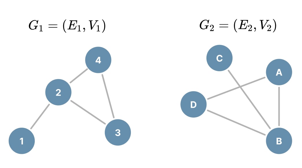

Figure 19. Two isomorphic graphs.

 

Weisfeiler-Lehman graph isomorphism test

The WL test¹⁵ is a well-known method to determine if two graphs are isomorphic. At the beginning, each node \(v_i \in V\) is assigned a unique label \(\ell_i^{(0)}\). Next, each node updates its label by aggregating the label multiset of its neighbors and its own label. To do this, an injective \(\text{Hash}\) function is used, guaranteeing that different inputs map to different outputs. The process is repeated until a number \(k\) of iterations is reached (or if we detect that the labels stopped to change).

\[\,\\ \ell_i^{(k+1)} = \text{Hash} \Big( \ell_i^{(k)},\; \{\!\{\ell_j^{(k)} | j \in \mathcal{N}_i\}\!\} \Big) \\\]

At the end of the algorithm, if the distribution of labels in the first graph is similar to the distribution of the second, this means that the two graphs may be isomorphic in the point of view of the WL test. Even if the WL test has a few limitations¹⁶, it can be used as a good baseline of expressiveness for GNN architectures.

 

Problem with some GNN architectures

As mentioned previously, GNNs follow an architecture based on the message passing mechanism. The \(\text{AGGREGATE}\) and \(\text{UPDATE}\) functions are respectively in charge of aggregating the neighborhood messages and updating the node features based on the aggregated messages. However, the choice of these functions is crucial because, depending on what is chosen, the GNN may not be able to keep the information about the structure of the graph.

For example, we can formulate the message passing mechanism of a GCN layer and a GraphSAGE¹⁷ layer as follows:

\[\text{GCN:} \quad h_i^{(l)} = \text{ReLU} \left( W \cdot \text{Mean} \left\{ h_j^{(l-1)} \;\middle|\; j \in \mathcal{N}_i \cup \{ i \} \right\} \right) \\ \text{GraphSAGE:} \quad a_i^{(l)} = \text{Max} \left( \left\{ \text{ReLU} \left( W \cdot h_j^{(l-1)} \right) \;\middle|\; j \in \mathcal{N}_i \right\} \right) \\\]

These two architectures use the \(\text{Mean}\) and \(\text{Max}\) functions to aggregate and update the neighborhood messages. But the problem is that these functions are poorly injective in terms of keeping the structure of the graph. So the GIN architecture proposes to use a combination of the \(\text{Sum}\) function and an MLP to ensure a message passing mechanism as expressive as the WL test

Also, the Figure 20 below from the GIN paper¹⁴ illustrates three cases in which the \(\text{Sum}\) passes the test of injectivity, but not the others. For each case, three isomorphic graphs are represented, and each node color corresponds to a unique value. If the function produces the same output for two or more graphs, then the function failed to distinguish isomorphic graphs. The functions are only computed on the neighbors of the center node (the empty one).

 

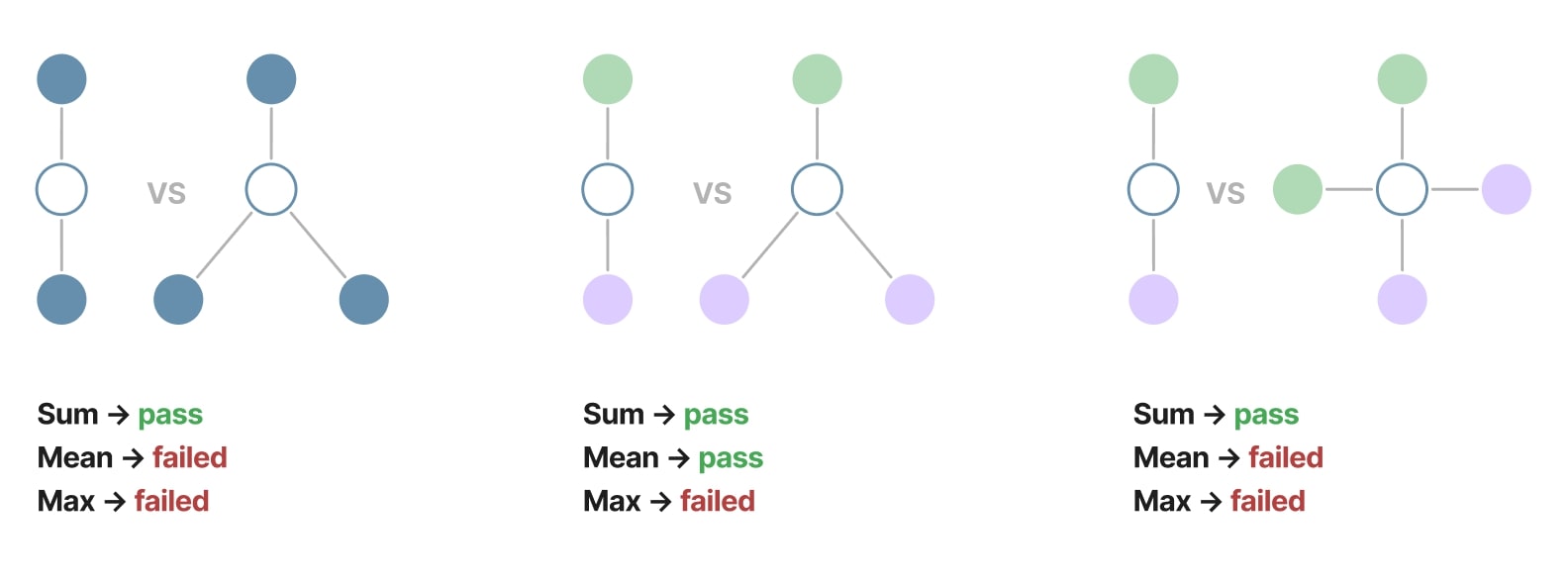
Figure 20. Sum, Mean and Max injectivity comparison.

 

This result doesn’t mean that the \(\text{Sum}\) is fully injective (it is not). However, it allows us to keep more information about the structure of graphs, and thus presents a better expressiveness. It is particularly beneficial to enforce this injectiveness property in the readout function, since it operates on the full graph, and lots of structural information could be lost with poorly injective readout functions.

 

Graph isomorphic layer

The proposed solution of the GIN architecture consists in summing the node features of the neighborhood. It is also possible to modify how the node itself is weighted in the aggregation with the hyperparameter \(\epsilon^{(l)}\). Some implementations of GIN even propose to make \(\epsilon^{(l)}\) learnable.

Next, an MLP is used to project the aggregated features in a latent space, instead of the traditional linear transformation. In fact, the MLP introduces several layers of linear transformation, biases, and non-linearity, increasing the expressiveness of the model:

\[\,\\ h_i^{(l)} = \mathrm{MLP}^{(l)}\left( (1+\epsilon^{(l)}) h_i^{(l-1)} + \sum_{j \in \mathcal{N}_i} h_j^{(l-1)} \right) \,\\ \,\\ \text{with} \quad h_G = \text{readout}(H^{(L)}) = \sum_{v_i \in V} h_i^{(L)}\]

Where:

• \(h_i^{(l)} \in \mathbb{R}^{d_n^{(l)}}\) is the node features at layer \(l\).
• \(\epsilon^{(l)} \in \mathbb{R}\) is the learnable hyperparameter for weighting the contribution of the node to its own aggregation/update.
• \(\mathrm{MLP}^{(l)}\) is a learnable multi-layer perceptron.
• \(\mathcal{N}_i \subset \mathbb{R}\) denote the set of neighbors of \(v_i\).

 

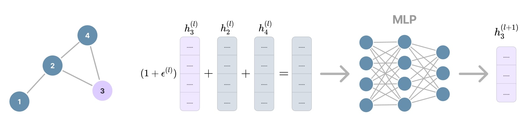
Figure 21. GIN layer details.

 

References

1. B. Sanchez-Lengeling, E. Reif, A. Pearce, A. B. Wiltschko. A Gentle Introduction to Graph Neural Networks. Distill 2021. ↩ ↩²

2. J. Zhou, G. Cui, S. Hu, Z. Zhang, C. Yang, Z. Liu, L. Wang, C. Li, M. Sun. Graph neural networks: A review of methods and applications. AI Open 2020. ↩ ↩² ↩³

3. V. P. Dwivedi, C. K. Joshi, A. T. Luu, Y. Bengio, X. Bresson. Benchmarking Graph Neural Networks. JMLR 2022. ↩

4. Z. Wang, S. Ji. Second-Order Pooling for Graph Neural Networks. IEEE 2020. ↩

5. Z. Wu, P. Jain, M. A. Wright, A. Mirhoseini, J. E. Gonzalez, I. Stoica. Representing Long-Range Context for Graph Neural Networks with Global Attention. NeurIPS 2021. ↩

6. J. Gilmer, S. S. Schoenholz, P. F. Riley, O. Vinyals, G. E. Dahl. Neural message passing for quantum chemistry. ICML 2017. ↩

7. K. Xu, C. Li, Y. Tian, T. Sonobe, K. Kawarabayashi, S. Jegelka. Representation Learning on Graphs with Jumping Knowledge Networks. ICML 2018. ↩

8. T. N. Kipf, M. Welling. Semi-Supervised Classification with Graph Convolutional Networks. ICLR 2017. ↩

9. M. Defferrard, X. Bresson, P. Vandergheynst. Convolutional Neural Networks on Graphs with Fast Localized Spectral Filtering. NeurIPS 2016. ↩

10. F. K. R. Chung. Spectral Graph Theory. AMS 1997. ↩

11. P. Veličković, G. Cucurull, A. Casanova, A. Romero, P. Liò, Y. Bengio. Graph Attention Networks. ICLR 2018. ↩

12. A. Vaswani, N. Shazeer, N. Parmar, J. Uszkoreit, L. Jones, A. N. Gomez, Ł. Kaiser, I. Polosukhin. Attention is All You Need. NeurIPS 2017. ↩

13. S. Brody, U. Alon, E. Yahav. How Attentive are Graph Attention Networks?. ICLR 2022. ↩

14. K. Xu, W. Hu, J. Leskovec, S. Jegelka. How Powerful are Graph Neural Networks?. ICLR 2019. ↩ ↩²

15. B. Y. Weisfeiler, A. A. Lehman. A Reduction of a Graph to a Canonical Form and an Algebra Arising during this Reduction. Nauchno-Technicheskaya Informatsia 1968. ↩

16. K. Sandra. Power and limits of the Weisfeiler-Leman algorithm. Aachen 2020. ↩

17. W. L. Hamilton, R. Ying, J. Leskovec. Inductive Representation Learning on Large Graphs. NeurIPS 2017. ↩