Introduction to Uncertainty Quantification for Deep Learning Models
Objectives and key references
-
This tutorial is aimed at giving a global overview of uncertainty quantification. Examples and methods are mainly oriented towards deep learning, classification and medical image processing. It does not give the tools to handle uncertainty quantification in practice, but the concepts to understand what is manipulated and how to evaluate it.
-
The introduction and modeling parts are strongly inspired by Hüllermeier et al. article, 2021 1 and the methods for quantification and evaluation are based on Lambert et al., 2024 2. Note that there is a recent review (2026) on uncertainty quantification methods for deep learning 3.
Summary
Introduction
Why quantifying uncertainty?
Deep learning models have achieved remarkable performance in a wide range of tasks. However, these models typically produce point predictions. In many real-world applications, such as medical diagnosis, autonomous driving or climate forecasting, knowing how reliable a prediction is can be just as important as the prediction itself. In this tutorial, we will only consider predictive uncertainty, in the sense of the uncertainty given an input sample.
Uncertainty quantification aims to provide a measure of confidence or reliability associated with model outputs. This is useful at two levels:
- when the model is deployed, it supports decision-making. For example, it can help to catch model failure, to redirect the predictions to human experts, or for the expert to discard the prediction. It can also guide active learning strategies.
- when the model is “under construction”, it helps evaluating a model and its limitations. It can also directly be used in some training strategies.
Sources and types of uncertainty
Uncertainty in machine learning predictions arises from multiple sources, which are often categorized into two main types 4.
Aleatoric uncertainty (AU) reflects the inherent randomness or noise in the data generation process. It is also referred to as “conflict” in classification, as it comes from an ambiguity between different classes. For example, it can arise from:
- the fact that measurement is a partial view of the true phenomenon;
- randomness of the true phenomenon itself;
- measurement noise in sensors;
- ambiguity in labeling…
This uncertainty is also sometimes called “irreducible uncertainty” because it cannot be reduced simply by collecting more data, since it is tied to the stochastic nature of the observations.
Epistemic uncertainty (EU), on the other hand, arises from a lack of knowledge about the true model, also referred to as “ignorance”. It reflects uncertainty in the model parameters or structure. It is related to all the sources of approximation needed because the perfect predictor is intractable (Figure 1):
- the choice of a model family \(\mathcal{H}\) in which the optimal predictor \(h^*\) is not the theoretical optimal predictor \(f_1^*\);
- learned solution \(\tilde{h}\) from an optimization process that does not align with the optimal \(h^*\);
- a possible difference between training distribution and real-world distribution that shifts the optimal predictor (sometimes called “distributional uncertainty”).
Unlike aleatoric uncertainty, epistemic uncertainty can often be reduced by gathering more informative data or improving the model.
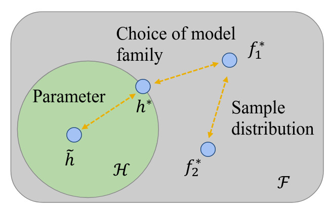
Figure 1. Visualization of various model uncertainty sources [He et al., ACM Comput. Surv., 2026]¹.
This distinction has an interest both theoretically and in practice. Theoretically, as illustrated later in Quantifying uncertainty, it exists mathematical decomposition of predictive uncertainty into two terms that can be linked to these two concepts. This distinction also leads to the design of different modeling techniques to capture different aspects of uncertainty.
In practice, when a prediction has high uncertainties, it triggers different actions 5.
- If AU is high, the clinician has the confirmation that it is a difficult sample, that the input data is ambiguous. He can run other tests to clear up the ambiguity. For the data scientist, it means it can be interesting to add other sources of information (other modalities, metadata, physics etc.) to the model.
- If EU is high, the clinician knows the prediction is not reliable, the model may fail on this input. It also means this data is of interest to further train the model. For the data scientist, it means the model needs to be more general, for example by adding data (new relevant samples, augmentations, …).

Figure 2. Illustration of the distinction between aleatoric and epistemic uncertainties [inspired from Hüllermeier et al., Mach. Learning, 2021].
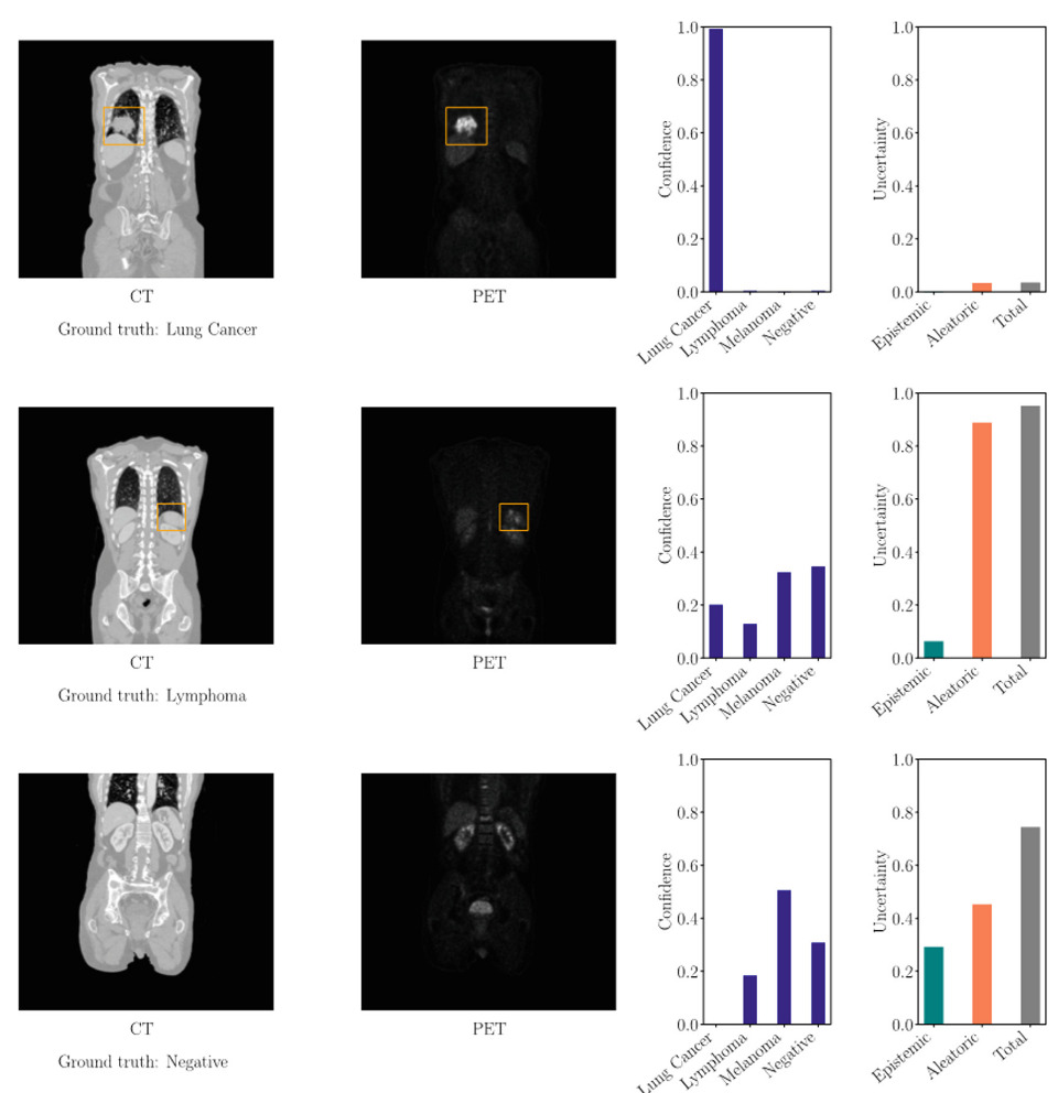
Figure 3. Examples of probabilistic predictions and uncertainty quantification (ensemble with entropy) results on a whole-body PET/CT dataset, with orange boxes surrounding the tumors identified by the physicians [Löhr et al., AIME, 2024].
These two types of uncertainty are general concepts that help highlighting the different sources of uncertainty, but their distinction can be blurry. The ambiguity needs to be cleared up in each specific context 1. These uncertainty are also strongly linked, as adding a dimension can decrease AU but increase EU (Figure 5), or having more samples can increase AU but decrease EU (Figure 4).
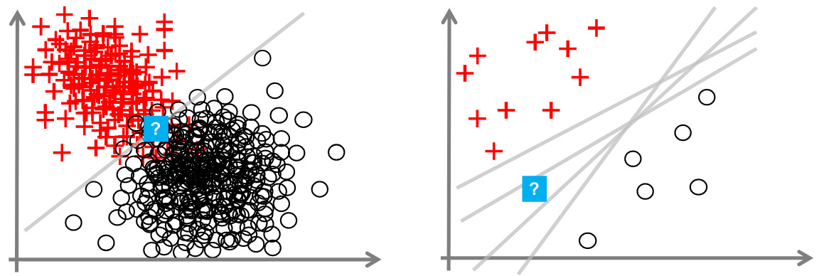
Figure 4. Adding data may reduce EU but can also increase AU. [Hüllermeier et al., Mach. Learning, 2021].
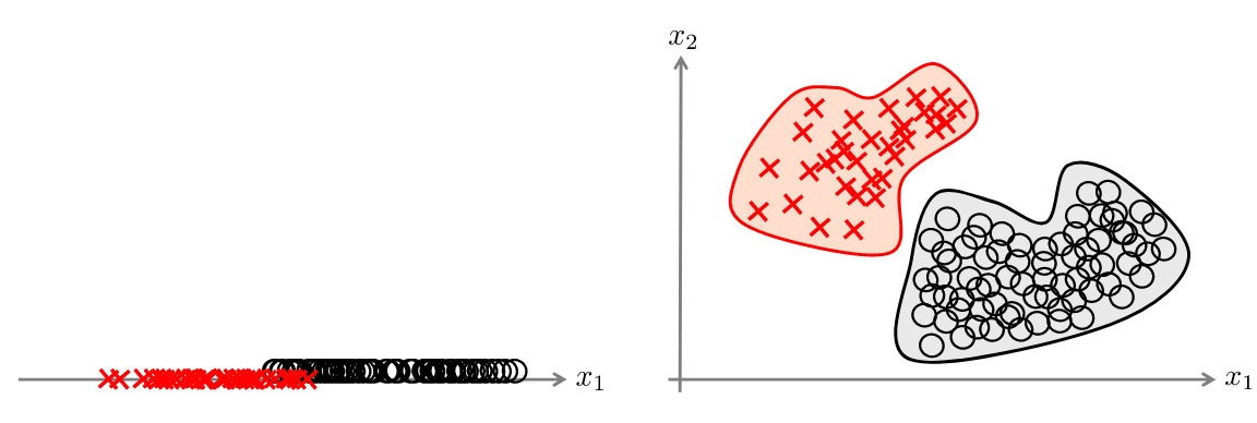
Figure 5. Adding a dimension may reduce AU but can also increase EU. [Hüllermeier et al., Mach. Learning, 2021].
Modeling uncertainty
Bayesian inference
Uncertainty are often characterized thanks to probabilities, and in particular in the Bayesian framework. Modeling uncertainty as distributions is in fact pretty natural in the field. This is why I will develop here this framework. We assume that we have a training set \(\mathcal{D}\) which contains N samples drawn independently from a distribution \(p\) on \(\mathcal{X} \times \mathcal{Y}\).
- Uncertainty in the data (aleatoric) Given an instance \(x_q\), the associated outcome \(y\) is not necessarily certain i.e. the best that we can obtain is a distribution:
We want to find a predictor \(f : \mathcal{X} \longrightarrow \mathcal{Y}\) that would best fit the data regarding an objective function \(l\) (induction):
\[f^*(x):=\text{argmin}_{ŷ\in\mathcal{Y}}\int_\mathcal{Y}l(y,\hat{y})dP(y|x)\]- Uncertainty in the model (epistemic) To do so, we only have access to an hypothesis space \(\mathcal{H}\), (with predictors \(h: \mathcal{X} \longrightarrow \mathcal{Y}\)) of models and we optimize a model by leveraging true labels to minimize the risk \(R\) under the objective function:
and we would like to obtain the best model in this space:
\[h^* = \text{argmin}_{h\in\mathcal{H}}R(h)\]However, we only have access to a finite number of elements, thus we often choose to minimize the empirical risk:
\[\hat{h} = \text{argmin}_{h\in{\mathcal{H}}} \frac{1}{N} \sum_{i=1}^N l(h(x_i), y_i)\]The total model uncertainty refers to the discrepancy between \(f^*\) and \(ĥ\). If we assume that the hypothesis space covers the optimal predictor (\(f^*=h^*\)), we can model the uncertainty due to approximation by the optimizer by a distribution \(\mathcal{Q}\) over the space \(\mathcal{H}\).
And beyond…
The Bayesian framework is not the only way to model uncertainty… As we can think about it as modelling ignorance, other frameworks are compatible, such as version space learning, where we consider a set of the predictors that are plausible on the train set rather than a distribution. A visualization of this diversity of methods is shown Figure 6.
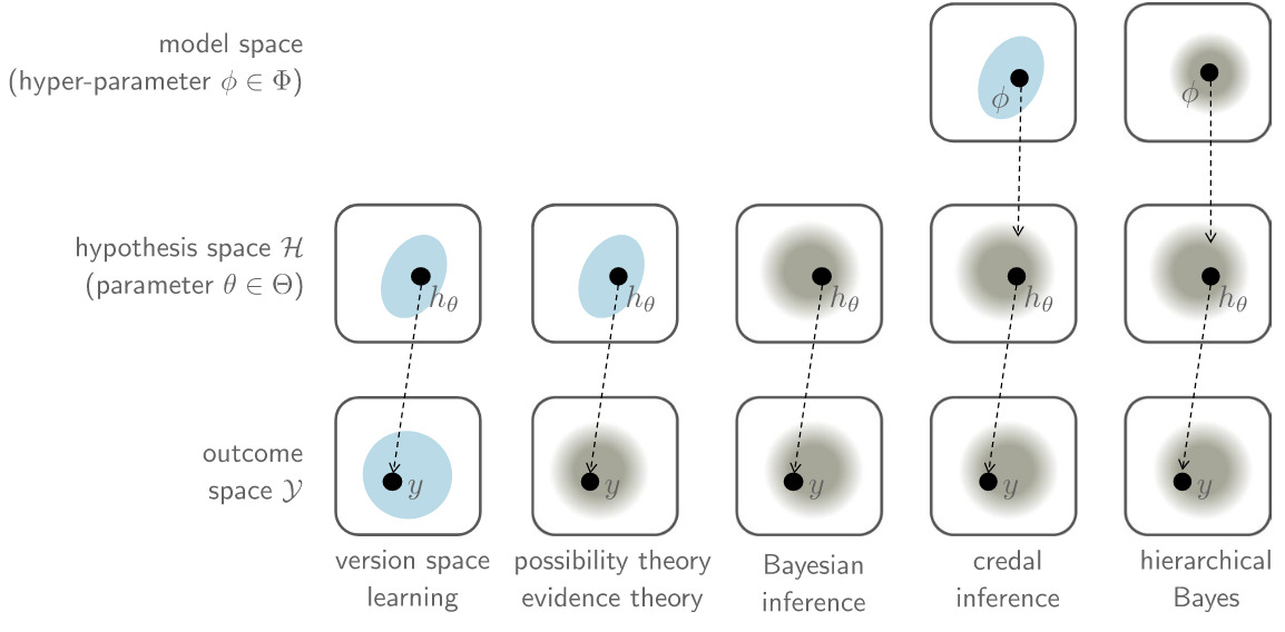
Figure 6. Set-based versus distributional knowledge representation on the level of predictions, hypotheses, and models. Representation as sets are blue forms, whereas representation in terms of distribution are in gray shading [Hüllermeier et al., Mach. Learning, 2021].
Quantifying uncertainty
Nice, we have modelled uncertainty… but in practice, we want a quantity that will translate this uncertainty, to be able to manipulate it and interpret it. This part first illustrates the kind of properties we want depending on the task, then lists several methods of quantification, focusing on deep learning. The objective of this part is not to present the different methods in detail, but to make a list so that you can investigate the one that seems the most adapted to your problem.
Different goals for different tasks
Because machine learning is used for different tasks, uncertainty is described in different ways.

Figure 7. Different quantities for different tasks.
A first approach for classification: softmax probabilities
A natural and widely used way to quantify uncertainty in classification tasks is through the output of the softmax layer. For a given input, the model produces a probability distribution over classes, and the maximum softmax probability is often interpreted as a measure of confidence. Intuitively, a prediction is considered uncertain when the probability mass is spread across several classes, and confident when one class dominates. However, this interpretation can be misleading: modern neural networks tend to be overconfident, even when they are wrong. As shown by Guo et al. (2017), softmax probabilities are often poorly calibrated, meaning that predicted probabilities do not reflect true correctness likelihood. As a result, additional techniques such as temperature scaling can be used a posteriori to obtain calibrated uncertainty estimates.
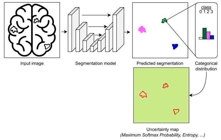
Figure 8. Illustration of UQ based on softmax probabilities [Lambert et al., 2024]
Bayesian Neural Networks (BNNs)
BNNs treat the network weights as probability distributions instead of fixed values. During inference, predictions are obtained by integrating over these distributions, capturing uncertainty in the model parameters 6.
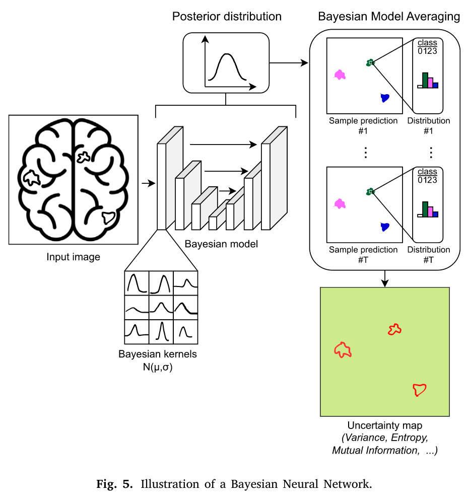
Figure 9. Illustration of UQ based on BNNs [Lambert et al., 2024]
Uncertainty type
Both
Advantages
- Principled probabilistic framework
- Captures both AU and EU naturally
- Strong theoretical grounding
Limitations
- Depends on the choice of the prior distribution over weights (often Gaussian)
- Computationally expensive
- Difficult to scale to large networks
- Approximate inference (e.g., variational) can be inaccurate
Monte Carlo dropout (MCDO)
MCDO keeps dropout active during inference and performs multiple stochastic forward passes. The variability in predictions approximates a posterior distribution over outputs. It is a practical approximation to Bayesian inference in deep learning 7.
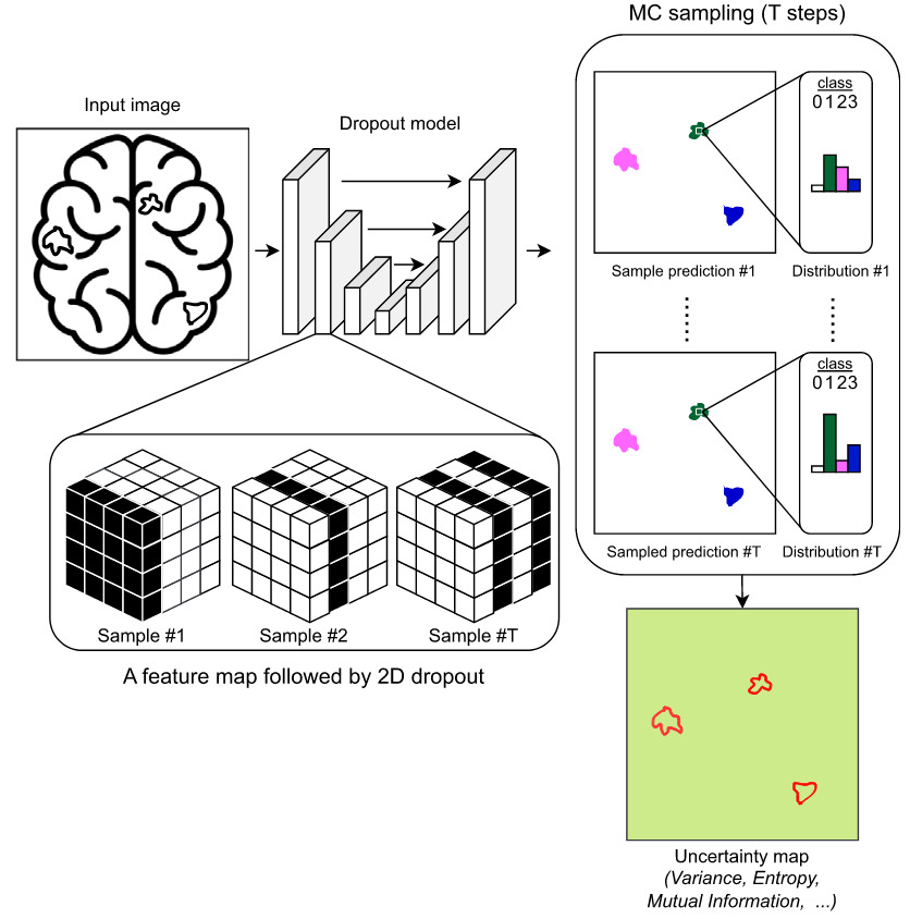
Figure 10. Illustration of UQ based on Monte Carlo dropout [Lambert et al., 2024]
Uncertainty type
Primarily EU, but can capture AU indirectly if modeled in the output
Advantages
- Easy to implement (just reuse dropout)
- Low overhead compared to full BNNs
- Scalability
- Works with existing trained models
Limitations
- Depends on the choice of a dropout probability (but some methods to fix it in the reference paper)
- Requires multiple forward passes (slow inference)
- Quality of uncertainty depends on dropout design
- Less theoretically precise than true BNNs
Ensemble methods
Multiple models are trained independently (different initializations, data splits, or architectures). Predictions are aggregated, and disagreement between models reflects uncertainty 8. This diversity approximates epistemic uncertainty.
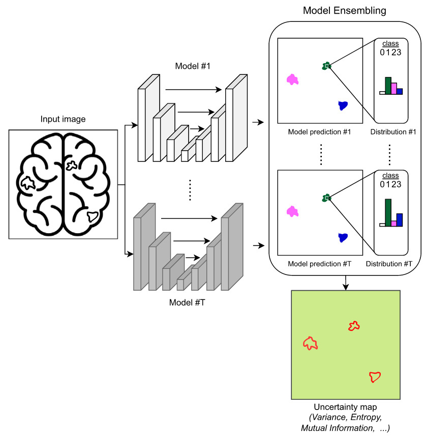
Figure 11. Illustration of UQ based on Deep Ensembles [Lambert et al., 2024]
Uncertainty type
Both, but especially strong for EU
Advantages
- Strong empirical performance
- Simple and robust
- Captures model uncertainty well
- Can boost performances
Limitations
- Uncertainty performance depends on how well model variability is represented by the technique
- High training and memory cost (multiple models)
- Slower inference
- Not a fully Bayesian method
Test-time augmentation (TTA)
TTA applies multiple transformations (e.g., flips, rotations) to the same input at inference time. Predictions are aggregated across augmented versions, and variation reflects sensitivity to input perturbations. This provides a measure of uncertainty related to data variability 9 10.
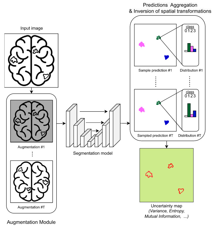
Figure 12. Illustration of UQ based on TTA [Lambert et al., 2024]
Uncertainty type
Primarily AU
Advantages
- Easy to apply without retraining
- Improves robustness and accuracy
- Captures input-related variability
Limitations
- It can be hard to identify meaningful augmentations in some contexts
- Limited to predefined transformations
- Adds inference cost
- Does not capture model uncertainty (EU)
Point on aggregation for these methods
With Monte Carlo Dropout, Ensemble methods, Test-time Augmentations and BNNs, you obtain T predictions for the same input, with T a chosen number of passes giving you T predictive probability vectors \((p_t(y|x))_{t=1}^T\). First, the final prediction is often obtained py the predictive mean:
\[\bar{p}(y|x) = \frac{1}{T} \sum_{t=1}^T p_t(y| x)\]Then, there is two main methods to obtain quantities reflecting uncertainty.
- Entropy decomposition: the entropy of this predictive mean reflects the total uncertainty. This uncertainty can be decomposed in two terms:
where the mutual information is defined as:
\[\underbrace{\mathrm{MI}}_{\text{EU}} = \underbrace{H\big(\bar{p}\big)}_{\text{Total}} - \underbrace{\mathbb{E}[H(p_t)]}_{\text{AU}}\]This mutual information is equivalent to the mean of the Kullback-Leibler divergences between the predictions and the mean prediction. It assumes that if the model is certain, there will not be too much difference (in the sense of KL-divergence) between the predictions.
The AU is the mean of the entropy of all the predictions: it assumes the model is certain if the predictions are mainly certain.

Figure 13. Illustration of the assumptions behind entropy decomposition between EU and AU.
- Variance decomposition: in the case of regression, the variance is a common way to describe the dispersion of prediction. It is less used for classification as it is harder to define variance for the discrete distributions. Here, the decomposition between AU and EU is obtained thanks to the law of total variance.
Evidential deep learning
Evidential learning models predict parameters of a probability distribution over possible outputs (e.g., Dirichlet or Normal-Inverse-Gamma) 11. Instead of sampling, the network directly outputs evidence about predictions and their uncertainty. It separates data noise from model confidence in a single forward pass.
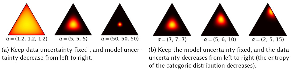
Figure 14. Example of Dirichlet distribution for 3 classes. The model will predict the parameters of a Dirichlet distribution, which gives a distribution over possible distribution for the point prediction. [He et al., 2026]
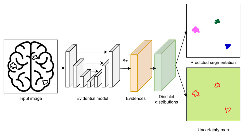
Figure 15. Illustration of UQ based on evidential learning [Lambert et al., 2024]
Uncertainty type
Both AU and EU
Advantages
- Single forward pass (efficient)
- No sampling required
- Explicit decomposition of uncertainty
Limitations
- Training can be unstable
- Sensitive to loss design and regularization
- May produce overconfident estimates if mis-specified
Conformal Prediction (CP)
CP provides prediction sets (or intervals) with guaranteed coverage under minimal assumptions 12. Several methods exists but the main one for classification uses calibration data to quantify uncertainty without modifying the underlying model (split CP). The uncertainty is expressed as prediction regions rather than probabilities.
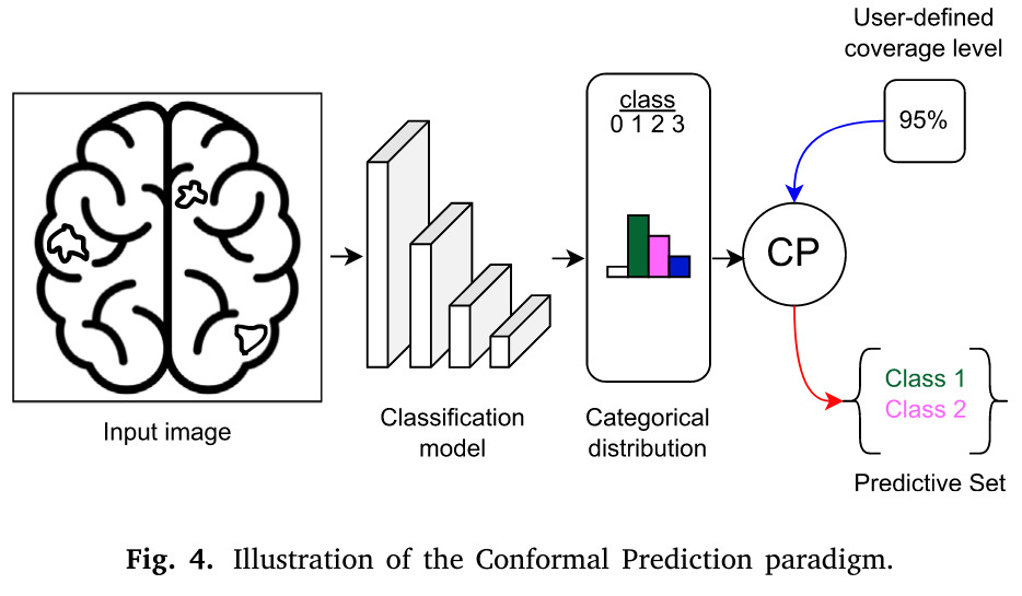
Figure 16. Illustration of UQ based on conformal prediction [Lambert et al., 2024]
Uncertainty type
Typically AU, but can reflect both depending on the model and setup
Advantages
- (Distribution-free) coverage guarantees, with few hypothesis on data
- Model-agnostic
- Easy to wrap around existing models
- Can be combined with another uncertainty quantification method
Limitations
- Produces sets/intervals (not full distributions)
- Can be conservative (wide intervals)
- Requires separate calibration dataset
- Needs to define a measure of uncertainty for the problem
- Assumes data is exchangeable
When going through the literature of conformal prediction, be really cautious when manipulating coverage guarantees. In fact, the main idea behind conformal prediction is that we have statistical guarantees at a given degree of confidence (for exemple the probability of the true prediction to be in the interval is of 95%). But this guarantee is in general on the marginal coverage, i.e.on the joint distribution on the data, and does not hold for a specific draw of a dataset either for an individual input. Ideally would like a conditional coverage which is stronger as it holds for any input. Some methods a=have this property in practice but with additional assumptions on data distribution.
Overview of uncertainty quantification methods used in medical imaging
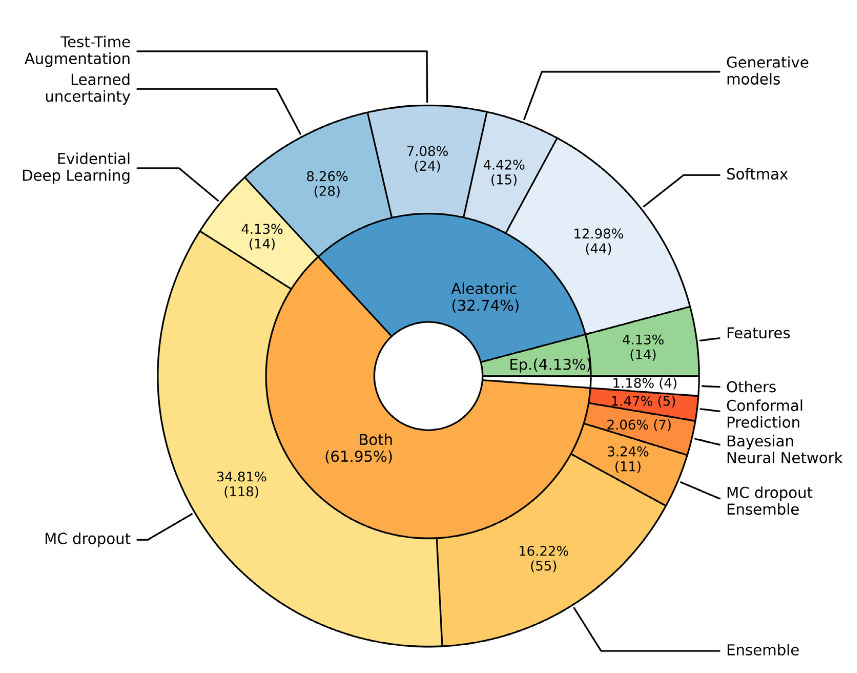
Figure 17. Distribution of UQ methods used for medical images between 2015 and 2023 (218 papers) [Lambert et al., 2024]
Evaluating uncertainty
We want to answer the question: does the uncertainty quantification method has desirable properties in practice ? These properties can be different depending on the context.
Metrics
-
Qualitative evaluation: the expert observes most uncertain and certain sample to see if its consistent with its intuition.
-
Calibration 13: a calibrated model is a model for which a prediction with an uncertainty score of \(c\) means that the probability of error is \(c\). To evaluate the calibration of a model, we group (either quantiles or fixed intervals) the predictions of the test set by their uncertainty scores and observe the error ratios in each group. The Expected Calibration Error (ECE) is the distance of this curve to the ideal curve. Note there exists also the Negative Log-Likelihood score.
-
Coverage error: estimating the difference between the empirical coverage of the test set and the desired coverage, for methods that fix a coverage (like CP).
-
Out-Of-Domain (OOD) detection: trying the model on out-of-domain datasets and evaluating if the uncertainty quantities are higher as expected, i.e. if they allow to detect OOD data.
-
Error detection: as uncertainty is often used to support decision-making by identifying predictions to dismiss, this scenario is simulated by removing the samples sorted by decreasing uncertainty and observing if the task performances are improving.
Adding evaluation of reliability
There is a claim to enforce model evaluation by diversifying what is evaluated. For instance, Hesse et al. 14 proposed an evaluation with 9 metrics, and they were able to compare methods and highlight their strengths and weaknesses on other metrics than pure task performance. Hedrycks et al. 15 have corroborated that pre-training can improve model robustness and uncertainty.
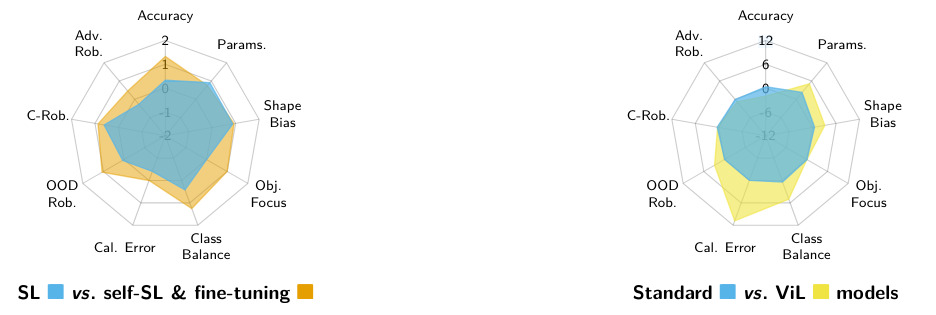
Figure 17. Evaluation of groups of models according to 9 evaluation criteria [Hesse et al., 2025]
References
-
E. Hüllermeier and W. Waegeman, “Aleatoric and epistemic uncertainty in machine learning: an introduction to concepts and methods,” Mach Learn, vol. 110, no. 3, pp. 457–506, Mar. 2021, doi: 10.1007/s10994-021-05946-3. ↩ ↩2
-
B. Lambert, F. Forbes, S. Doyle, H. Dehaene, and M. Dojat, “Trustworthy clinical AI solutions: A unified review of uncertainty quantification in Deep Learning models for medical image analysis,” Artificial Intelligence in Medicine, vol. 150, p. 102830, Apr. 2024, doi: 10.1016/j.artmed.2024.102830. ↩
-
W. He, Z. Jiang, T. Xiao, Z. Xu, and Y. Li, “A Survey on Uncertainty Quantification Methods for Deep Learning,” ACM Comput. Surv., vol. 58, no. 7, p. 179:1-179:35, Feb. 2026, doi: 10.1145/3786319. ↩
-
A. Kendall and Y. Gal, “What Uncertainties Do We Need in Bayesian Deep Learning for Computer Vision?,” in Advances in Neural Information Processing Systems, Curran Associates, Inc., 2017. Available: https://proceedings.neurips.cc/paper/2017/hash/2650d6089a6d640c5e85b2b88265dc2b-Abstract.html ↩
-
T. Löhr, M. Ingrisch, and E. Hüllermeier, “Towards Aleatoric and Epistemic Uncertainty in Medical Image Classification,” in Artificial Intelligence in Medicine, J. Finkelstein, R. Moskovitch, and E. Parimbelli, Eds., Cham: Springer Nature Switzerland, 2024, pp. 145–155. doi: 10.1007/978-3-031-66535-6_17. ↩
-
C. Blundell, J. Cornebise, K. Kavukcuoglu, and D. Wierstra, “Weight Uncertainty in Neural Network,” in Proceedings of the 32nd International Conference on Machine Learning, PMLR, Jun. 2015, pp. 1613–1622. Available: https://proceedings.mlr.press/v37/blundell15.html ↩
-
Y. Gal and Z. Ghahramani, “Dropout as a bayesian approximation: Representing model uncertainty in deep learning,” in international conference on machine learning, PMLR, 2016, pp. 1050–1059. Available: https://proceedings.mlr.press/v48/gal16.html?trk=public_post_comment-text ↩
-
B. Lakshminarayanan, A. Pritzel, and C. Blundell, “Simple and Scalable Predictive Uncertainty Estimation using Deep Ensembles,” in Advances in Neural Information Processing Systems, Curran Associates, Inc., 2017. Available: https://proceedings.neurips.cc/paper_files/paper/2017/hash/9ef2ed4b7fd2c810847ffa5fa85bce38-Abstract.html ↩
-
G. Wang, W. Li, M. Aertsen, J. Deprest, S. Ourselin, and T. Vercauteren, “Aleatoric uncertainty estimation with test-time augmentation for medical image segmentation with convolutional neural networks,” Neurocomputing, vol. 338, pp. 34–45, Apr. 2019, doi: 10.1016/j.neucom.2019.01.103. ↩
-
M. S. Ayhan and P. Berens, “Test-time Data Augmentation for Estimation of Heteroscedastic Aleatoric Uncertainty in Deep Neural Networks,” in 1st Conference on Medical Imaging with Deep Learning, Amsterdam, The Netherlands, 2018. ↩
-
M. Sensoy, L. Kaplan, and M. Kandemir, “Evidential Deep Learning to Quantify Classification Uncertainty,” in Advances in Neural Information Processing Systems, Curran Associates, Inc., 2018. Available: https://proceedings.neurips.cc/paper/2018/hash/a981f2b708044d6fb4a71a1463242520-Abstract.html ↩
-
A. N. Angelopoulos and S. Bates, “A Gentle Introduction to Conformal Prediction and Distribution-Free Uncertainty Quantification,” Dec. 07, 2022, arXiv: arXiv:2107.07511. doi: 10.48550/arXiv.2107.07511. ↩
-
C. Guo, G. Pleiss, Y. Sun, and K. Q. Weinberger, “On Calibration of Modern Neural Networks,” in Proceedings of the 34th International Conference on Machine Learning, PMLR, Jul. 2017, pp. 1321–1330. Available: https://proceedings.mlr.press/v70/guo17a.html ↩
-
R. Hesse, D. Bağcı, B. Schiele, S. Schaub-Meyer, and S. Roth, “Beyond Accuracy: What Matters in Designing Well-Behaved Image Classification Models?,” Transactions on Machine Learning Research, Aug. 2025. Available: https://openreview.net/forum?id=E7HDtLCoT6 ↩
-
D. Hendrycks, K. Lee, and M. Mazeika, “Using Pre-Training Can Improve Model Robustness and Uncertainty,” in Proceedings of the 36 th International Conference on Machine Learning, Long Beach, California, 2019, pp. 1–10. ↩